Анализ статистических данных в MINITAB - Моделирование временного ряда (Time Series Forecasting)
Подождите немного. Документ загружается.

Time Series Forecasting 213
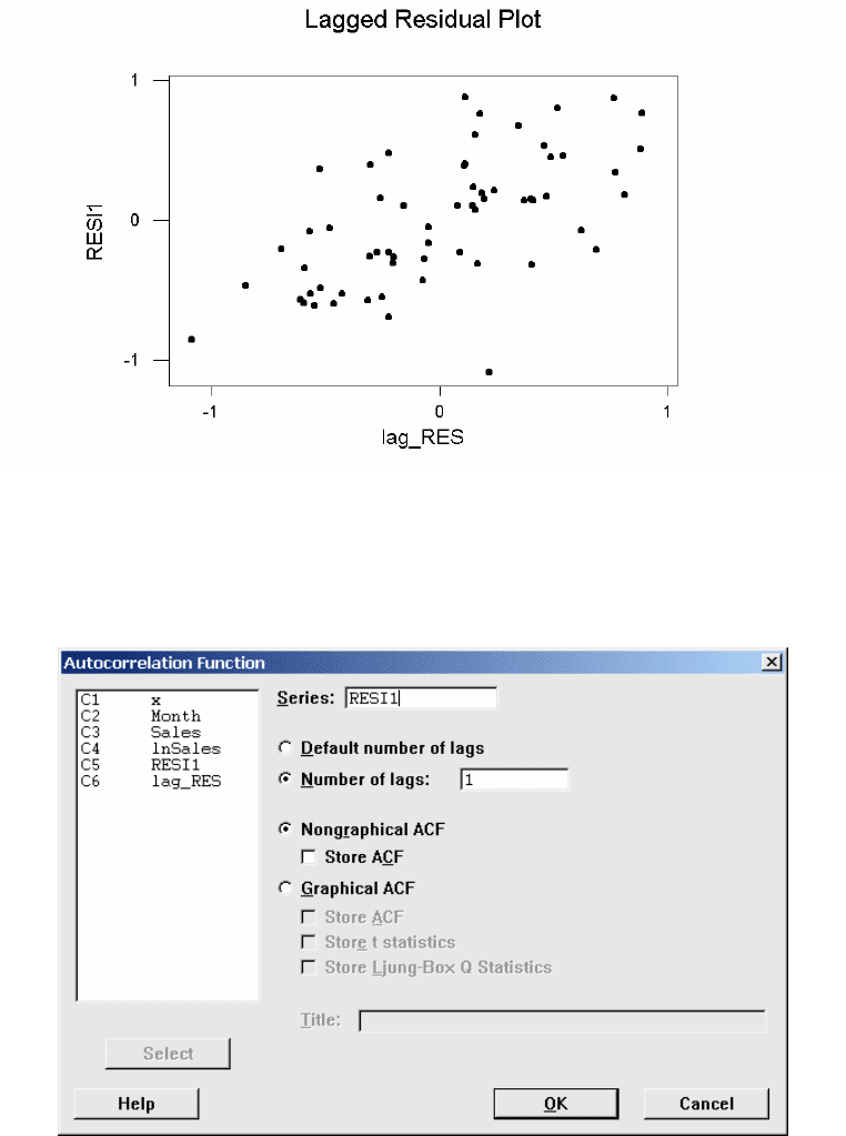
Minitab can be used to calculate the autocorrelation for the lagged residuals lagged. Select
Stat h Time Series h Autocorrelation
from the menu. In the dialog box, enter the column containing the residuals under Series. Specify one
as the number of lags to use instead of the default and check Nongraphical ACF.
Minitab calculates the autocorrelation to be 0.614.
Autocorrelation Function: RESI1
ACF of RESI1
-1.0 -0.8 -0.6 -0.4 -0.2 0.0 0.2 0.4 0.6 0.8 1.0
+----+----+----+----+----+----+----+----+----+----+
1 0.614 XXXXXXXXXXXXXXXX
214 Chapter 13
Moving Average Models
Moving average models use the average of the last several values of the time series to forecast the next
value. Example 13.12 of PBS calculates moving averages for quarterly JCPenny sales data with the
moving average forecast model based on a span of k = 4. The data are available in TA13_001.MTW.
Select
Stat h Time Series h Moving Average
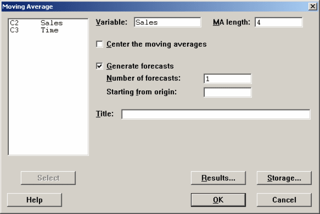
from the menu. In the dialog box, enter the column containing the sales data under Variable. In the
Moving Average (MA) length box, enter the span k = 4. Check Generate forecasts and enter one for
Number of forecasts.
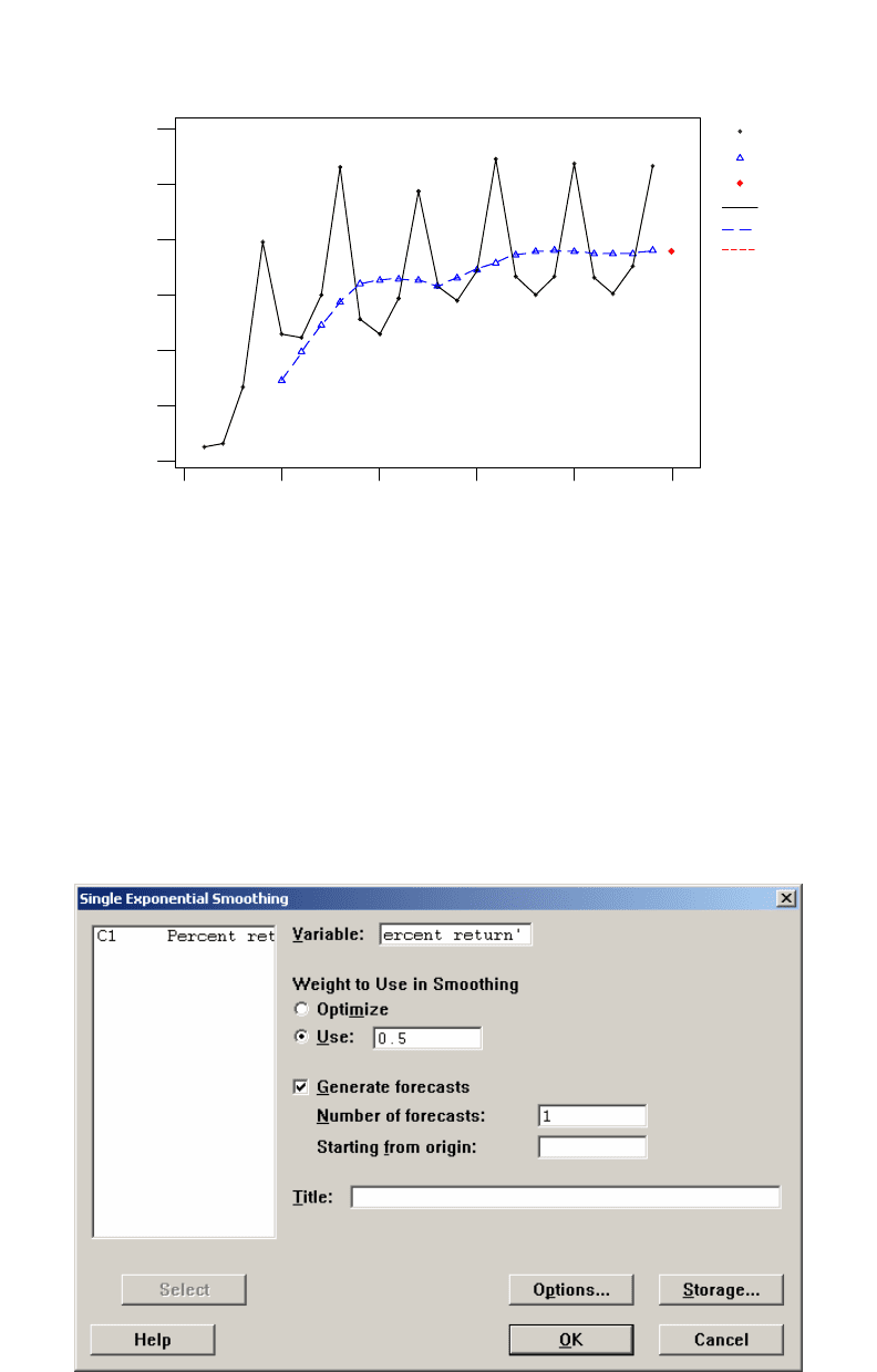
Minitab calculates the forecasted value for the first quarter of 2002 and generates a time series plot.
Moving average
Data Sales
Length 24.0000
NMissing 0
Moving Average
Length: 4
Accuracy Measures
MAPE: 10
MAD: 809
MSD: 1072724
Row Period Forecast Lower Upper
1 25 8001 5970.98 10031.0
Time Series Forecasting 215
Actual
Predicted
Forecast
Actual
Predicted
Forecast
0 5 10 15 20 25
4200
5200
6200
7200
8200
9200
10200
Sales
Time
Moving Average
4
10
809
72724
Moving Average
.5.0=w
Length:
MAPE:
MAD:
MSD:
10
Exponential Smoothing Models
Example 13.15 of PBS uses an exponential smoothing model to forecast monthly returns on Philip
Morris stock. The data are available in TA01_010.MTW. In this example, we use the smoothing con-
stant
Select
Stat h Time Series h Single Exp Smoothing
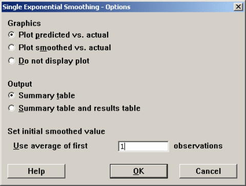
from the menu. In the dialog box, enter the column containing the time series under Variable. Under
Weight to Use in Smoothing, choose Use to enter a specific weight, then type 0.5 in the text box.
216 Chapter 13
With the Use option, Minitab uses the average of the first six observations for the initial smoothed value
by default. You can change this default by specifying a different value in the Single Exponential
Smoothing - Options sub-dialog box.
Minitab forecasts a 0.1939% return for Philip Morris stock in August 2001.
Single Exponential Smoothing
** Note ** Zero values of Yt exist; MAPE calculated only for non-zero Yt
Data Percent retu
Length 134.000
NMissing 0
Smoothing Constant
Alpha: 0.5
Accuracy Measures
MAPE: 226.740
MAD: 7.288
MSD: 81.604
Row Period Forecast Lower Upper
1 135 0.193989 -17.6624 18.0504
Time Series Forecasting 217
100500
Actual
Predicted
Forecast
Actual
Predicted
Forecast
20
0
-20
Percent retu
Time
MSD:
MAD:
MAPE:
Alpha:
Smoothing Constant
81.604
7.288
226.740
0.500
Single Exponential Smoothing
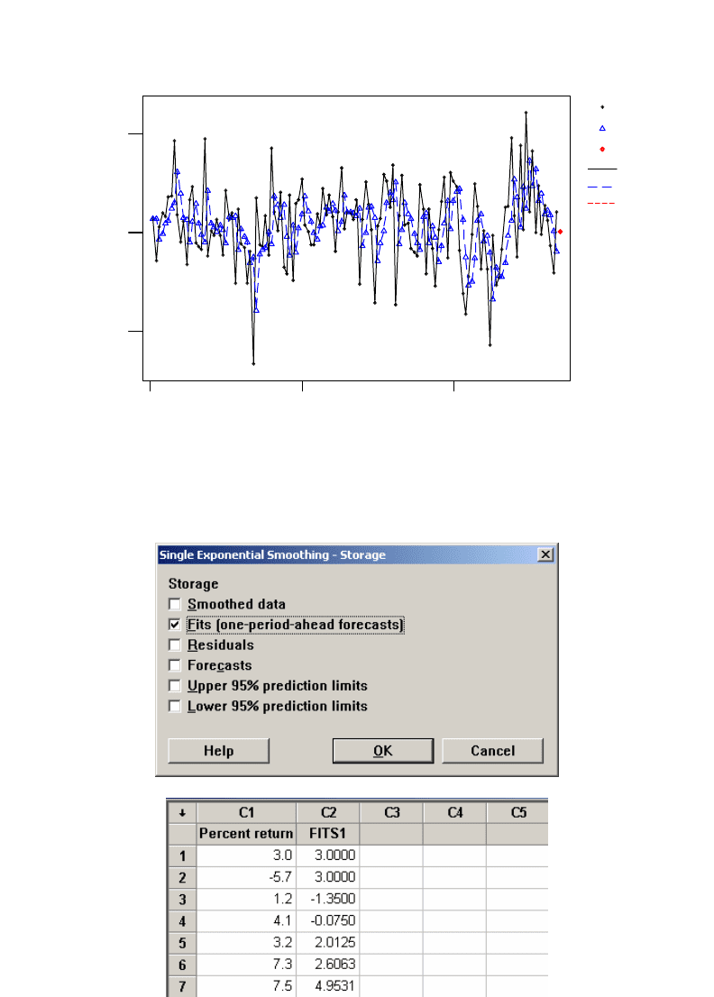
To calculate all past forecasts as shown in Example 13.15 of PBS, click on the storage button and select
Fits (one-period-ahead-forecasts).
218 Chapter 13
EXERCISES
13.1 Table 13.1 of PBS and TA13_001.MTW contain retail sales for JCPenney in millions of dol-
lars. The data are quarterly beginning with the first quarter of 1996 and ending with the fourth
quarter of 2001.
(a) Before plotting these data, inspect the values in the table. Do you see any interesting
features of JCPenney quarterly sales?
(b) Now, select
Stat h Time Series h Time Series Plot from the menu to make a time
plot of the data. Be sure to connect the points in your plot to highlight patterns.
(c) Is there an obvious trend in JCPenney quarterly sales? If so, is the trend positive or
negative?
(d) Is there an obvious repeating pattern in the data? If so, clearly describe the repeating
pattern.
13.3 In Exercise 13.1, you took a first look at the data in Table 13.1 of PBS and TA13_001.MTW.
Use Minitab to further investigate the JCPenney sales data.
(a) Select
Stat h Regression h Regression from the menu and find the least-squares line
for the sales data. Use
as the values for the explanatory variable with X = 1
corresponding to the first quarter of 1996, X = 2 corresponding to the second quarter of
1996, etc.
K,3,2,1
(b) The intercept is a prediction of sales for what quarter?
(c) Interpret the slope in the context of JCPenney quarterly sales.
(d) Using the equation of least-squares line, forecast sales for the first quarter of 2002 and
for the fourth quarter of 2002.
(e) Which forecast in part (d) do you believe will be more accurate when compared to ac-
tual JCPenney sales? Why?
13.4 Table 13.2 of PBS and TA13_002.MTW display the time series of number of Macintosh com-
puters shipped in each of eight consecutive fiscal quarters. Select
Stat h Time Series h Time
Series Plot
from the menu to make a time plot of the data. With only eight quarters, a strong
quarterly pattern is hard to detect. Select
Stat h Regression h Regression from the menu and
calculate the least-squares regression line for predicting the number of Macs shipped (in thou-
sands of units). The explanatory variable Time simply takes on the values
1
in time
order. Next, add indicator variables for first, second, and third quarters to the linear trend
model. Call these indicator variables X1, X2, and X3, respectively. Select
Stat h Regression
h Regression
from the menu to fit this multiple regression model.
8,,3,2, K
(a) Write down the estimated trend-and-season model.
(b) Explain why no indicator variable is needed for fourth quarters.
(c) What does the ANOVA F test indicate about this model?
13.5 In Exercise 13.1, you made a time plot of the
JCPenney sales data in Table 13.1 of PBS and
TA13_001.MTW. Sales seem to follow a pattern of ups and downs that repeats every four
quarters. Add indicator variables for first, second, and third quarters to the linear trend model.
Call these indicator variables X1, X2, and X3, respectively. Select
Stat h Regression h Re-
gression
from the menu to fit this multiple regression model.
(a) Write down the estimated trend-and-season model.
(b) Explain why no indicator variable is needed for fourth quarters.
Time Series Forecasting 218a
(c) Does the intercept still predict sales for a specific quarter? If so, what quarter? Com-
pare the estimated intercept of this model with that of the trend-only model. Given the
pattern of seasonal variation, which appears to be the better estimate?
(d) Using the equation of the trend-and-season model, forecast sales for the first quarter of
2002 and for the fourth quarter of 2002.
(e) Compare your forecasts to the same forecasts based on the trend-only model of Exer-
cise 13.3.
13.6 In Exercise 13.4, you fit a linear trend-only model to the Macs shipped time series in
TA13_002.MTW. Starting with this trend-only model, incorporate seasonality factors for each
quarter.
(a) Select
Stat h Time Series h Decomposition from the menu to calculate the seasonal-
ity factor for each quarter. Since the data is quarterly data, use a seasonal length of 4 in
the dialog box.
(b) Average the four seasonality factors. Is this average close to one? If so, interpret the
seasonality factor for first quarters.
(c) Select
Graph h Plot from the menu and make a scatterplot of seasonality factor versus
quarter. Connect the points to see the general pattern of seasonal variation. Also, draw
a horizontal line at the average of the four seasonality factors.
13.7 In Exercise 13.3, you fit a linear trend-only model to the JCPenney sales data. Starting with
this trend model, we want to incorporate seasonality factors to account for the pattern that re-
peats every four quarters.
(a) Select Stat h Time Series h Decomposition from the menu to calculate the seasonal-
ity factor for each quarter. Since the data is quarterly data, use a seasonal length of 4 in
the dialog box.
(b) Average the four seasonality factors. Is this average close to one? If so, interpret the
seasonality factor for fourth quarters.
(c) Select
Graph h Plot from the menu and make a scatterplot of seasonality factor versus
quarter. Connect the points to see the general pattern of seasonal variation. Also, draw
a horizontal line at the average of the four seasonality factors.
(d) Using the linear trend-only model and the seasonality factors, forecast sales for the first
quarter of 2002 and for the fourth quarter of 2002.
(e) Compare your forecasts to the same forecasts based on the trend-only model of Exer-
cise 13.3.
(f) Compare your forecasts to the same forecasts based on the trend-and-season model of
Exercise 13.5.
13.16 Select
Stat h Time Series h Decomposition from the menu to calculate the seasonality factor
for each quarter
for the JCPenney sales data. (Since the data is quarterly data, use a seasonal
length of four).
(a) In the dialog box, click on the Storage button and check Seasonally adjusted data to
calculate the seasonally adjusted JCPenney sales time series.
(b) Select
Stat h Time Series h Time Series Plot from the menu to make a time plot of
the original sales data with the seasonally-adjusted sales data superimposed. In the dia-
log box, fill in two rows as the Graph variables: the original time series and the season-
ally adjusted time series. Click on the Frame button and choose Multiple Graphs. In the
sub-dialog box, choose Overlay graphs on the same page and click OK.
218b Chapter 13
(c) Did seasonally-adjusting JCPenney’s sales data smooth the time series to the degree
that seasonally-adjusting the sales data in Figure 13.7 of PBS did? What does this im-
ply about the strength of the seasonal pattern in these two time series?
13.17 In Exercise 13.3, a linear trend-only model was fit to the JCPenney sales data. Using the re-
siduals from this model, look for evidence of autocorrelation.
(a) Select
Stat h Time Series h Time Series Plot from the menu and make a time plot of
the residuals. Describe any pattern you see in this plot.
(b) Select
Stat h Time Series h Lag from the menu and calculate the lagged residuals.
Select
Graph h Plot from the menu and plot the residuals versus the lagged residuals.
Select
Stat h Time Series h Autocorrelation from the menu and calculate the corre-
lation between successive residuals. Do we have evidence of autocorrelation?
13.18 In Exercise 13.5, a trend-and-season model was fit to the JCPenney sales data. Using the re-
siduals from this model, look for evidence of autocorrelation.
(a) Select
Stat h Time Series h Time Series Plot from the menu and make a time plot of
the residuals. Describe any pattern you see in this plot.
(b)
Select Stat h Time Series h Lag from the menu and calculate the lagged residuals.
Select
Graph h Plot from the menu and plot the residuals versus the lagged residuals.
Select
Stat h Time Series h Autocorrelation from the menu and calculate the corre-
lation between successive residuals. Do we have evidence of autocorrelation?
13.22 The United States Department of Agriculture (USDA) tracks prices received by Montana farm-
ers for winter wheat crops. The prices are tracked monthly in dollars per bushel.
EX13_022.MTW has the wheat prices time series beginning in July 1929 and ending with Oc-
tober 2002 (880 months). Use Minitab to analyze this time series.
(a) Select
Stat h Time Series h Time Series Plot from the menu and make a time plot of
the wheat prices time series.
(b) Describe any important features of the time series. Be sure to comment on trend, sea-
sonal patterns, and significant shifts in the series.
(c) Select
Stat h Time Series h Moving Average from the menu to calculate 12-month
moving averages and generate a time series plot. In the dialog box, enter the Moving
Average (MA) length = 12.
(d) Select
Stat h Time Series h Moving Average from the menu to calculate 120-month
moving averages and generate a time series plot. In the dialog box, enter the Moving
Average (MA) length = 120.
(e) Compare the 12-month and 120-month moving averages. Which features of the wheat
prices time series does each capture? Which features does each smooth?
13.29 Example 1.7 of PBS looked at the trend and seasonal variation in the average monthly price of
oranges. Figure 1.7 of PBS is a time series plot of the data. The data is found in
FG01_007.MTW.
(a) Select
Stat h Time Series h Single Exp Smoothing from the menu to calculate expo-
nential smoothing models using smoothing constants of w = 0.1, 0.5, and 0.9.
(b) Comment on the smoothness of each exponential smoothing model in part (a). Which
model would be best for forecasting monthly ups and downs in orange prices?
Time Series Forecasting 218c
(c) Select Stat h Time Series h Single Exp Smoothing from the menu to calculate and
compare forecasts for January 2001 orange prices for each of the models in part (a).
Which model provided the most accurate forecast? (The actual value of the orange
prices time series for January 2001 is 224.2.)
(d) Update your data by appending the January 2001 observed value of 224.2. Now select
Stat h Time Series h Single Exp Smoothing from the menu to forecast the February
2001 orange price with each of the models from part (a). Which model provided the
most accurate forecast? (The actual value of the orange prices time series for February
2001 is 229.6.)
