Ahsan A. Two Phase Flow, Phase Change and Numerical Modeling

Подождите немного. Документ загружается.

Thermal Approaches to Interpret

Laser Damage Experiments 3

responsible for laser-induced damage in dielectrics. Unlike the standard 0.5 value of x that

has been demonstrated in a lot of materials by both experimental (Stuart et al., 1996) and

simple physical considerations (Bliss, 1971; Feit & Rubenchik, 2004; Wood, 2003), LID in KDP

exhibits a lower value of x that is close to 0.35 at 3ω (Adams et al., 2005; Burnham et al.,

2003). A ﬁrst attempt has been made by Feit and co-workers to explain this deviation from 0.5

(Feit & Rubenchik, 2004; Trenholme et al., 2006). Hereafter, in the tradition of the state-of-the-

art above-mentioned thermal modeling, an introduction to the general model is done. This

model that takes into account all relevant physical mechanisms involved in LID in order to

predict x values that depart from the standard 0.5. Under a few assumptions, this is achieved

by coupling a Drude model, the Mie theory and Thermal diffusion. The resulting model

hereafter referred to as DMT is presented in Sec. 2.1.1. It allows to predict the values of F

and x with respect to the optical constants of the plasma (see Sec. 2.1.3). The inverse problem

(Gallais et al., 2004) is considered in order to determine the modeling physical parameters

from experimental data. It permits to draw up conclusions about the electronic plasma

density. Further, the evolution of the scaling law exponent is studied with respect to the laser

pulse duration interval that is used to evaluate it.

2.1.1 Thermal modeling and absorption efﬁciency

Since LID consists of a set of pinpoints distributed randomly within the bulk (Adams et al.,

2005), the model considers the heating of a set of plasma balls whose radius varies from a few

nanometers to hundreds of nanometers (Feit & Rubenchik, 2004). The main assumptions of

the model are the following :

• continuity of the size distribution, i.e. it exists at least one sphere for each size,

• since it deals with a plasma, a high thermal conductivity of the absorbing s phere is

assumed. It follows that the temperature is constant inside the plasma,

• the absorption efﬁciency is independent of time, i.e. it is assumed that the plasma reaches

its stationary state in a time much shorter than the laser pulse duration,

• when the critical temperature T

is reached at the end of the pulse, an irreversible damage

occurs,

• the physical parameters do not depend on the temperature.

The heating model for one sphere is based on the standard diffusion equation (Feit &

Rubenchik, 2004; Hopper & Uhlmann, 1970) that can be written in spherical symmetry as :

∂T

∂t

∂

∂r

∂T

∂r

) (1)

where T is the temperature, r is the radial coordinate and D is the bulk thermal diffusivity

deﬁned as D

ρC

with λ

, ρ, C being the thermal conductivity, the density and the speciﬁc

heat capacity of the KDP bulk respectively. Eq. (1) is solved under the following initial and

boundary conditions :

i. at t

= 0, T = T

= constant ∀ r,whereT

is the initial ambient temperature set to 300 K,

ii. T tends to T

when r tends to inﬁnity,

iii. the following enthalpy conservation at the interface between the bulk and the absorber is

considered:

4π

∂T

∂t



r=a

= I

abs

(m, y)πa

+ 4πa

∂T

∂r



r=a

(2)

219

Thermal Approaches to Interpret Laser Damage Experiments

4 Will-be-set-by-IN-TECH

where a, ρ

and C

are the radius, the density and the speciﬁc heat capacity of the absorber

respectively. Q

abs

(m, y) is deﬁned as the absorption efﬁciency that can be evaluated

through the Mie theory (Van de Hulst, 1981). m is the complex optical index of the absorber

related to the one of the bulk and y is the size parameter. Finally, I

is the laser intensity that

is assumed to be constant with respect to time in order to correspond to an experimental

top hat temporal proﬁle.

Eq. (1) can be solved in the Laplace space (Carslaw & Jaeger, 1959) and the use of the initial

and boundary conditions leads to the following solution for r

= a :

(a, τ)=T

abs

√

4Dτ

4λ

ξ(U, A) (3)

with

(U, A)=

1 − X



(

) − X

φ(

)



(4)

where U



, X = U +

√

−1andA =

√

4κτ

are dimensionless. Note that ξ(U, A)

is a function that gives acoount for the material properties. The notation κ =

3λ

4ρ

is also

introduced and has units of a thermal diffusivity, but mixes the properties of the bulk and

the absorber. The function φ is deﬁned as φ

(z)=1 − exp(z

) erfc(z) where erfc is the

complementary error function. Also, the ﬂuence can be written as F

= I

τ which allows Eq. 3

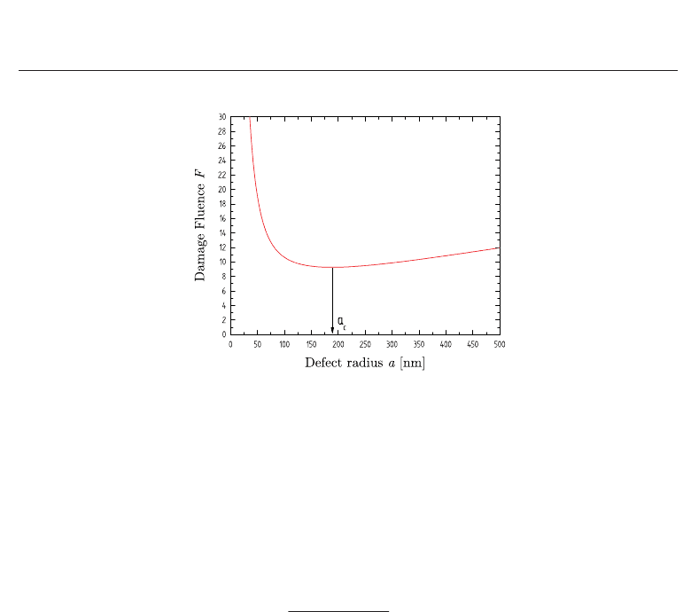
to be re-formulated. The plot of F as a function of a exhibits a minimum (Hopper & Uhlmann,

1970) (see Fig. 1) and since the existence of at least one absorber of size a is assumed, the critical

ﬂuence necessary to reach the critical temperature T

(set to 10000 K in all the calculations

(Carr et al., 2004)) can thus be written as :

2λ

− T

)

abs

)

√

ξ(U, A

)

(5)

where a

is the radius that corresponds to the minimum ﬂuence to reach T

Moreover, for the case where Q

abs

does not depend on a, one can show from Eq. (5) and Fig. 1

that the critical ﬂuence reaches a minimum for the critical radius a

(τ)=2

√

κτ B(U) (6)

where B is a function of U.ItcanbeshownthatB

(∞)=1andB(0)  0.89. Elsewhere, the

function B

(U) has to be evaluated numerically. If Q

abs

does not depends on a,thenx = 1/2.

It is worth noting that the value of x can be refound from considerations about the enthalpy

conservation at the interface.

The second step consists in showing by simple considerations how the introduction of the Mie

theory permits to deviate from the standard x

= 1/2value. Fromthattheory,Q

abs

depends

on the sphere radius. More precisely, one can reasonably write Q

abs

∝ a

where δ ∈ [−1; 1].

= −1 corresponds to the case a

> λ and large values of the imaginary part k of the optical

index (typically a few unities as for metals) whereas δ

= 1 corresponds to the Rayleigh regime

( a

 λ). As above mentioned, a

is a function of the pulse duration that can be written as

∝ τ

where γ is close to 1/2. It follows that F

∝ τ

1/2−δγ

with −1/2 ≤ δγ ≤ 1/2 and

therefore x lies in the range

[0; 1].

220

Two Phase Flow, Phase Change and Numerical Modeling

Thermal Approaches to Interpret

Laser Damage Experiments 5

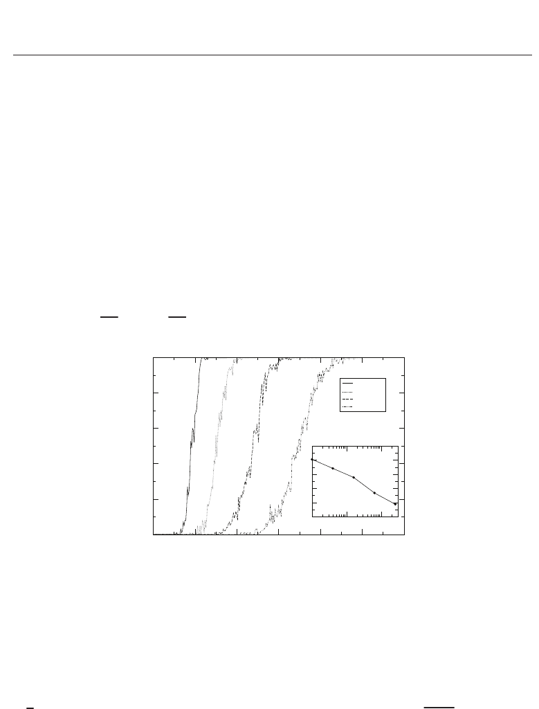
Fig. 1. Evolution of the damage ﬂuence F

as a function of the defect size a. A minimum is

obtained for a

= a

which is associated to the critical ﬂuence F

2.1.2 Determination of the plasma optical indices within the Drude model framework

Since the laser absorption is due to a plasma state, for which free electrons oscillate in the

laser electric ﬁeld and undergo collisions with ions, the optical indices of the plasma can be

derived from the standard Drude model with damping (see for example Hummel (2001)). In

that framework, the response of the electron gas to the external laser electric ﬁeld is given by

the following complex dielectric function :

= 1 −

ω(ω −i/τ

col l

)

−iε

(7)

In this expression, ω

is the electron plasma frequency given by ω

=(n

/ε

∗

)

1/2

where

is the free electrons density and m

∗

is the effective mass of the electron. τ

col l

stands for

the collisional time, i.e. the time elapsed between two collisions with ions. The dielectric

function is linked to the complex optical index m

= n − ik by the relation m

= ε.It

follows that ε

= n

− k

and ε

= 2nk.Inthecasewherem and hence ε are known,

the characteristic parameters of the plasma n

and τ

col l

can be determined by inversing

Eq. (7). The laser-induced electron density cannot exceed a critical value n

above which

the plasma becomes opaque. This critical density is determined setting ω

to ω,whichleads

to n

= m

∗



. In the next section, we will see that it is of interest to know the values

of the optical index satisfying the physical requirement n

≤ n

(or equivalently ω

≤ ω)

appearing in laser-induced experiments. By setting n

to n

,thecouples(ε

, ε

) have to satisfy

(ε

−1/2)

+ ε

=(1/2)

that is nothing but the equation of a circle centered at (1/2, 0) and

of radius 1/2. Each point inside the circle satisﬁes the required condition n

≤ n

2.1.3 Results

A description of the procedure that is used to compute all physical parameters of interest for

the present paper is done ﬁrst. For given pulse duration and

(n, k) values, the plot of the

ﬂuence required to reach the critical temperature T

as a function of the absorber radius – the

plot that exhibits a minimum a

(Feit & Rubenchik, 2004) – allows to determine the critical

221

Thermal Approaches to Interpret Laser Damage Experiments

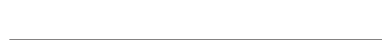
6 Will-be-set-by-IN-TECH

ﬂuence F

, i.e. the ﬂuence for which the ﬁrst damage appears. It is also possible to associate

the critical Mie absorption efﬁciency Q

abs

) evaluated for a = a

. In order to determine

the scaling law exponent x corresponding to a couple

(n, k), one only has to apply the last

procedure for different pulse durations. It is then assumed that one can write F

= Aτ

and

the values of the parameters A and x are determined with a ﬁtting procedure based on a

Levenberg-Marquardt algorithm (Numerical Recipies, n.d.).

Now, within this modeling framework, the optical constants of the plasma can be determined

by using experimental data that provide F

and x. To do so, by applying the above-described

procedure, the theoretical evolution of F

and x have been evaluated as a function of (n, k)

on Figs. 2 (a) and 2 (b) respectively. Fig. 2 (a) has been obtained with τ = 3 ns whereas,

for Fig. 2 (b), τ varies in the interval

[1. ns ; 10. ns] which is used experimentally (Burnham

et al., 2003). The particular behavior of F

can be explained in a simple way. From Eq. (5),

is proportional to 1/Q

abs

, Q

abs

being itself proportional to ε

= 2nk since it deals with

conditions close to the Rayleigh regime (Van de Hulst, 1981) (a

 100 nm and thus a/λ < 1)

and ε

 1. Iso-ﬂuence curves as shown on Fig. 2 (a) correspond to F

= const, that is to

say 1/Q

abs

= const and subsequently k ∝ 1/n. This hyperbolic behavior is all the more

pronounced that τ is short. As regards the scaling law exponent, the main feature appearing

on Fig. 2 (b) is that x depends essentially on k, this trend becoming more pronounced as k

goes up. Indeed, for large enough values of k whatever the value of n,theshapeofQ

abs

with respect to a remains almost the same that imposes the value of x. Now, the optical

constants can be determined from experimental data F

= 10 ± 1 J/cm

(Carr et al., 2004) and

= 0.35 ±0.05 (Burnham et al., 2003). The theoretical index range providing these two values

is obtained by performing a superposition of Figs. 2 (a) and 2 (b) as shown on Fig. 2 (c). In

addition, the intersection region is restricted by the above-mentioned condition ω

≤ ω.Since

the uncertainty on F

is relatively small, the shape of the intersection region is elongated. The

extremal points in the

(n, k) plane are roughly (0.16, 0.16) (n

= n

and τ

col l

= 3.50 fs) and

(0.40, 0.06) (n

= 0.84n

and τ

col l

= 3.27 fs). The optical index satisfying F

= 10 J.cm

−2

and

= 0.35 is (0.22, 0.12) (n

= 0.97n

and τ

col l

= 3.40 fs). Also, we ﬁnd values of n

and τ

col l

that are close to the plasma critical density and the standard femtosecond range respectively.

It is worth noting that the associated Mie absorption efﬁciency with the latter optical indices

is Q

abs

)=6.5 % where a

 100 nm. In order to compare to experiments where the ionized

region size is estimated to 30 μm (Carr et al., 2004) in conditions where the ﬂuence is twice the

critical ﬂuence (for such a high energy, the plasma spreads over the whole focal laser spot),

we have evaluated Q

abs

with the above found index and a = 30 μm.Inthatcase,Q

abs

 10 %

which is close to the 12 % experimental value (Carr et al., 2004). It is noteworthy that Q

abs

saturates with respect to a for such values of the optical index and absorber size.

2.2 Coupling statistics and heat tranfer

In order to characterize experimentally the resistance of KDP crystals to optical damaging,

a standard measurement consists in plotting the bulk damage probability as a function of

the laser ﬂuence F (Adams et al., 2005) that gives rise to the so-called S-curves. In order

to explain this behavior, thermal models based on an inclusion heating have been proposed

(Dyan et al., 2008; Feit & Rubenchik, 2004; Hopper & Uhlmann, 1970). In these approaches,

statistics (Poisson law) and inclusion size distributions are assumed. On the other hand,

pure statistical approaches mainly devoted to the onset determination and that do not take

into account thermal processes have been considered (Gallais et al., 2002; Natoli et al., 2002;

O’Connell, 1992; Picard et al., 1977; Porteus & Seitel, 1984). On the basis of the above-

222

Two Phase Flow, Phase Change and Numerical Modeling

Thermal Approaches to Interpret

Laser Damage Experiments 7

Fig. 2. (top left) Critical ﬂuence F

in J.cm

−2

as a function of n and k for τ = 3 ns.(topright)

Scaling law exponent x as a function of n and k for τ

∈ [1. ns; 10. ns]. (bottom) Intersection of

(a) and (b), the highlighted area delimits the region satisfying experimental data.

mentioned assumption of defects aggregation, this section proposes a model where Absorbing

Defects of Nanometric Size, hereafter referred to as ADNS, are distributed randomly and may

cooperate to the temperature rise ΔT through heat transfer within a given micrometric region

of the bulk that corresponds to an heterogeneity. Since this approach combines statistics

and heat transfer, it allows to provide the cluster size distribution, damage probability as a

function of ﬂuence, and scaling laws without any supplementary hypothesis. The present

section aims at introducing the general principle of this model and giving ﬁrst main results

that are compared with experimental facts. A particular attention has been payed to scaling

laws since they are very instructive in terms of physical mechanisms. More precisely, a

deviation from the standard τ

1/2

law has recently been observed within KDP crystals (Adams

et al., 2005) and this model (as the DMT one previously presented) also proposes a plausible

explanation of this fact based on thermal cooperation effects and statistics. Despite the 2D

and 3D representation was tackled (Duchateau, 2009; Duchateau & Dyan, 2007), this section

focuses on a one dimensional modeling that gives a good insight about physics and seems to

provide a nice counterpart to experimental tendencies.

This section is organized as follows: Sec. 2.2.1 deals with the model coupling statistics and

heat transfer. In a ﬁrst part, the principle of the approach is exposed. Secondly, numerical

223

Thermal Approaches to Interpret Laser Damage Experiments

8 Will-be-set-by-IN-TECH

predictions of the model are provided in terms of damage probability S-curves and temporal

scaling laws. Results are discussed and compared with experimental facts in Sec. 2.2.2.

2.2.1 Random distribution of absorbing defects

This model considers a set of ADNS that are distributed on a spatial domain. When a crystal

cell contains a defect, it is called an alterate cell which may absorb laser energy much more

efﬁciently than a pure cell crystal. Therefore, from heat transfer point of view, the alterate

cell may be seen as a very tiny source inducing temperature rising. This source of size a is

assumed to be close to the characteristic crystal cell dimension, i.e. one nanometer. Within a

1D framework, the domain of size Na, that is assumed to correspond to an heterogeneity, then

is composed of two kinds of cells. The temperature evolution is governed by the Fourier’s

equation:

∂T

∂t

= D

∂

∂x

ρC

ADNS

∑

i=1

Π(x − x

) (8)

where x

∈ [0, Na] stands for the position of ADNS or alterate cells whose number is n

ADNS

and A is the absorbed power per unit of volume. Material physical parameters such as thermal

diffusivity D and conductivity λ,densityρ or speciﬁc heat capacity C, linked by the relation

= λ/ρC, are assumed to remain constant in the course of interaction. The function Π is

deﬁned as follows:



(x)=1ifx ∈ [x −a/2; x + a/2]

Π(x)=0elsewhere

(9)

The way to distribute defects is addressed in the next paragraph. A general solution of (8) is

given by (Carslaw & Jaeger, 1959):

(x, t)=T

ADNS

∑

i=1

ΔT

(i)

(x, t) (10)

where T

= 300K is the initial temperature of the crystal and where the temperature rise

ΔT

(i)

(x, t) induced by one ADNS is solution of the following equation:

∂ΔT

(i)

∂t

= D

∂

ΔT

(i)

∂x

ρC

(x −x

) (11)

Now, since conditions are a



√

Dt (for D

KDP

= 6.5 × 10

−7

−1

and τ = 1ns,itleadsto

√

Dt  25nm), in order to deal with simple formula allowing fast numerical calculations, the

function Π

(x) is replaced by the Dirac delta function δ(x), i.e.it is imposed that the energy

absorbed by a ﬁnite-size defect is in fact absorbed by a point source. The ADNS then may

be seen as a heating point source. Within this framework, a good approximated solution of

Eq. (11) is given by:

(x, t)=

2λ







1/2

exp



−

4Dt



− x erfc



√





(12)

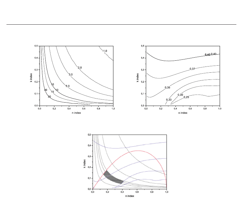
The reliability of this approximation has been checked by performing a full numerical

resolution of Eq. (8) based on a ﬁnite differences scheme. In order to illustrate the main

principle of the model, Fig. 3 plots the evolution of the temperature (10) as a function of the

1D spatial coordinate in a case for which n

ADNS

= 15, A/ρC = 10

K.s

−1

and τ = 1 ns.This

224

Two Phase Flow, Phase Change and Numerical Modeling

Thermal Approaches to Interpret

Laser Damage Experiments 9

300

400

500

600

700

800

900

1000

1100

1200

1300

1400

1500

1600

Temperature [K]

1000 1100 1200 1300 1400

1500

1600

Distance [nm]

Fig. 3. Spatial temperature evolution resulting from a particular random throwing. 15 ADNS

are present, A/ρC

= 10

K.s

−1

and τ = 1 ns are used. The temperature rise is enhanced

when several ADNS aggregate. Defects positions are shown by vertical arrows.

graph shows a characteristic spatial behavior where it clearly appears that cooperative effect

leads to a locally higher temperature.

From these calculations, it is then possible to construct a damage probability law. For a given

ﬂuence F,anumbern

dra w

of ADNS distribution are generated, and it is checked whether

or not each ADNS distribution induces a temperature higher than the critical temperature

.Letn

dam

be the number of ADNS conﬁgurations leading to T ≥ T

. Then, the damage

probability is simply given by P

(F)=n

dam

(F)/ n

dra w

. In order to plot the damage probability

as a function of ﬂuence, the source term of Eq. (11) has to be evaluated. Since the defect nature

is unknown, the absorbed power per unit of volume A cannot be evaluated theoretically thus

leading to an empirical evaluation from experimental data. From dimensional analysis, it can

be written that A

= ξF/lτ where ξ and l may be identiﬁed to a dimensionless absorption

efﬁciency and an effective cluster size respectively. In conditions where thermal diffusion is

not taken into account, the temperature rise induced by the laser pulse reads ΔT

= Δρ

/ρC

where Δρ

= ξ F/l and C = 0.023 × 900  2 J.K

−1

.cm

−3

are the absorbed energy per unit

of volume and the heat capacity per unit volume of KDP respectively. From black body

measurements (Carr et al., 2004), it turns out that the temperature rise associated with damage

induced by a 3ns laser pulse with F

 10J.cm

−2

is roughly 10000K. That allows to estimate the

unknown ratio ξ/l to about 2

×10

−1

. In fact, thermal diffusion processes take place, and

ξ/l must be higher. Therefore, we choose ξ/l

= 10

−1

and we will check in Sec. 2.2.2 that

it is consistent with experimental data. Since we are working within the Rayleigh regime for

which ξ ∝ l (defects clusters are assumed to be well smaller than λ

= 351nm), it is assumed

that ξ/l to remain almost unchanged when l varies. Also, the use of A

= 10

× F/τ as the

source term empirical expression of Eq. (11) in numerical calculations is done.

In following calculations, critical temperature is ﬁxed to T

= 5000 K (Carr et al., 2004). The

Laser-Induced Damage Threshold (LIDT) is then deﬁned as the value of the ﬂuence F

such

that the damage probability equals 10%. As usually in Physics, this choice indicates actually

the departure from perturbative conditions. It is worth noting that taking 5% or 20% will not

affect the main conclusions of this model.

225

Thermal Approaches to Interpret Laser Damage Experiments

10 Will-be-set-by-IN-TECH

2.2.2 Results

Let us begin with the 1D case. The damage probability as a function of the laser ﬂuence is

shownonFig.4forτ

= 250ps,1ns,4ns and 16ns. In all cases, we choose n

ADNS

= 100,

= 10000 and statistics is supported by 200 drawings. The general shape of curves exhibits

a standard behavior for which damage probabilities increase monotonically with the ﬂuence.

Further, calculations for τ

= 3 ns show that the LIDT is close to 9 J.cm

−2

that is in a good

agreement with Carr et al.’s experiment (Carr et al., 2004). Also, a posteriori,thisresultconﬁrms

the reliability of the evaluation of the coefﬁcient ξ/l that has been set to 10

−1

.Foragiven

pulse duration, probability becomes non-zero when, within at least one drawing, a group of

ADNS is sufﬁciently aggregated to form a cluster whose size and density are enough to reach

locally the critical temperature.

When the ﬂuence goes up, the critical temperature may be reached by smaller or less dense

cluster. Since they are in a larger number, the probability increases itself. A probability close

to one corresponds to the lowest cooperative effect, i.e. involving the smallest number of

ADNS around the place where T

≥ T

. This number is determined counting ADNS that

contribute signiﬁcantly to the place x

where T ≥ T

. To do so, the counting is made in the

range

− 4

√

Dτ, x

+ 4

√

Dτ]. It appears that, for a given pulse duration, the larger the

ﬂuence, the lesser the number of ADNS involved in the damage.

0.2

0.4

0.6

0.8

Damage Probability

Fluence [J.cm

-2

]

t = 250 ps

t = 1 ns

t = 4 ns

t = 16 ns

0.15

0.2

0.25

0.3

0.35

0.4

x-exponent

1 10 100

Pulse duration [ns]

Fig. 4. Evolution of the damage probability as a function of ﬂuence within the 1D model.

Four pulse durations are considered : τ

= 250ps,1ns,4ns and 16ns. Parameters are

ADNS

= 100 and N = 10000. 200 drawings have been performed for each ﬂuence.

Sub-ﬁgure displays the scaling law exponent as a function of the pulse duration (see text).

Now, les us focus on the inﬂuence of the pulse duration on the d amage probability curves

and, more precisely, the scaling law linking the ﬂuence to the pulse duration. Fig. 4 shows

clearly that the LIDT is shifted towards higher ﬂuence when τ increases. Actually, for long

pulse, the thermal diffusion process is more efﬁcient and more energy is needed to reach the

critical temperature for a given ADNS conﬁguration. For instance, the temperature rises as

√

τ (Carslaw & Jaeger, 1959) thus implying the scaling law F

√

/τ

.Inorderto

establish the scaling law in our model, it is assumed that F

=(τ

/τ

)

may be written.

The exponent x is determined from the knowledge of F

, F

, τ

and τ

. In fact, τ

= 4τ

stated and the x exponent is evaluated as a function of τ

ranging from 1 ns to 16 ns.The

values of F

and x are displayed for the above-mentioned values of τ in Table 1. Note that

more drawings than in Fig. 4 have been performed in order to determine F

with a correct

226

Two Phase Flow, Phase Change and Numerical Modeling

Thermal Approaches to Interpret

Laser Damage Experiments 11

numerical precision. It appears that x differs from the expected 1/2 value and takes values

[J.cm

−2

] x

τ = 250ps 3.85

= 1 ns 6.28 0.353

= 4 ns 9.80 0.321

= 16ns 14.60 0.288

Table 1. Critical ﬂuence and x-exponent as a function of the pulse duration

that depends on the pulse duration. For the sake of completeness, the values of x for a large

range of pulses ratios is plotted on sub-ﬁgure of Fig. 4. The evolution of x can be ﬁtted by the

empirical following expression:

= −α ln τ + β (13)

with α

= 2.92 × 10

−2

and β = 0.3592. The ﬁt error is close to 2% and may be due to

statistical uncertainties. We have checked that a different ratio τ

/τ

leads to the same general

expression of x but where the coefﬁcients α and β differ slightly. For a given ADNS spatial

conﬁguration, this behavior of x can be understood by the following consideration: for a

single ADNS, since ΔT ∝ τ

1/2

, the according scaling law reads F

∝ τ

1/2

. For a given pulse

duration, since several ADNS are involved, whose effective cluster size is non negligible in

comparison with the diffusion length, the temperature goes up faster than τ

1/2

and the scaling

law exponent is accordingly lower than 1/2. Now, when τ increases, since the contribution

length is proportional to

√

Dτ, more and more defects take part in the temperature rise. It is

like if the laser pulses sees different target sizes with respect to its duration. It then turns out

that less energy is needed than in a situation where all target components always contribute

for any interaction time. Consequently, the scaling law deviates from the standard x

= 1/2

value as the pulse duration goes up.

3. Evolutions of the thermal models and interpretation of the experiments

Sec. 2 has presented different thermal approaches capable to explain the most of usual

results of laser-induced damage in KDP crystals in the nanosecond range. Despite some

approximations, these models allow a good interpretation of the complex scenario of KDP

laser damage but do not include any polarization inﬂuence nor the presence of two laser

pulses with different wavelengths. In this section, the latter inﬂuences are thus addressed.

First, we focus on the effect of polarization on the laser damage resistance of KDP. Then we

will highlight the effect of multiple wavelength interacting with the crystal simultaneously

and the consequences on its resistance.

3.1 The effect of laser polarization on KDP crystal resistance: inﬂuence of the precursor

defects geometry

3.1.1 Experimental results at

1ω: laser damage density versus ﬂuence and Ω

Test protocol

Generally, laser damage tests yield to the Standard (ISO Standard No 11254-1:2000; ISO

Standard No 11254-2:2001, 2001). The so-called 1-on-1 procedure has been used here to test the

KDP crystal. Speciﬁc data treatments described in (Lamaignère et al., 2009) allow to extract

the bulk damage densities as a function of ﬂuence. This part interests more particularly in

the effect of the polarization on KDP crystals resistance. Then the Ω notation is introduced

227

Thermal Approaches to Interpret Laser Damage Experiments

12 Will-be-set-by-IN-TECH

as the angle between the polarization of the incident laser beam and the propagation axis.

In substance, Ω =0

◦

corresponds to the case where the laser polarization



E is collinear to the

ordinary axis of the crystal. When Ω =+90

◦



E is collinear to the extraordinary axis of the

crystal.

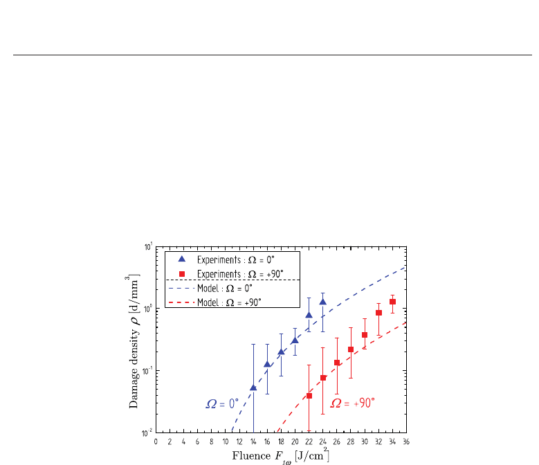
Evolution of the laser damage density versus ﬂuence

Fig. 5 presents the evolution of the laser damage density as a function of 1ω ﬂuence. Tests

have been performed for two orthogonal positions of the crystal, i.e. (a) the laser polarization

along the ordinary axis (blue triangles), (b) the laser polarization along the extraordinary axis

(red squares).

Fig. 5. Evolution of the laser damage density as a function of the 1ω ﬂuence. Blue triangles

correspond experimental results for the ordinary position (Ω =0

◦

) and red squares to

extraordinary position (Ω =90

◦

). Modeling results are represented in dash lines, respectively

for each test positions. Modeling results are discussed in Sec. 3.1.3. Damage densities evolve

as a power law of the ﬂuence.

According to Fig. 5, results clearly appear different between the two positions as we can

estimate a shift of about 10 J/cm

. This implies a factor 1.4 - 1.5 on the ﬂuence at constant

damage density.

Laser damage density versus Ω at 1ω

Studying the laser damage density as a function of the rotation angle Ω has been carried out

to investigate a potential effect due to ﬂuence. It is worth noting that rotating the crystal is

equivalent to turning the beam polarization. This test has been performed for two different

ﬂuences F

1ω

(i.e.at19J/cm

and 24.5 J/cm

). Note that the choice of these F

1ω

test ﬂuences

allows scanning damage probabilities in the whole range [0 ; 1]. Fig. 6 illustrates the damage

density as a function of Ω. Red squares and blue triangles respectively correspond to tests

carried out at F

1ω

= 24.5 J/cm

and at F

1ω

=19J/cm

Fig. 6 highlights the inﬂuence of crystal orientation on LID. To address this point, one may

interest in the variations of the damage density as a function of Ω. In the range [0

◦

,90

◦

], apart

from the points referenced by the black arrows (see explanations after), it can be observed

228

Two Phase Flow, Phase Change and Numerical Modeling