Agoston M.K. Computer Graphics and Geometric Modelling: Mathematics

and the equation for the rotation R about the origin through the angle -q is

Let C be the curve deﬁned by (3.60). Then the curve C≤=RT(C) has equation

(3.62)

and we are done.

Next, we use the eigenvalue approach. The eigenvalues are the roots of equation

(3.49), which reduces to

in this case. To solve for the eigenvectors for eigenvalues 25 and 100 we must solve

that is,

respectively. The solutions for the ﬁrst equation are x = (4/3)y, so that u

= (4/5,3/5) is

a unit eigenvector for eigenvalue 25. The solutions for the second equation are x =

(-3/4)y, so that u

= (-3/5,4/5) is a unit eigenvector for eigenvalue 100. The sub-

stitution speciﬁed by equation (3.51) would then again give us equation (3.62). It

corresponds to the same rotation R described above.

One point that one needs to be aware of when using the eigenvalue approach is

that there is some leeway as to our choice of eigenvectors. Our only real constraint is

that the orthonormal basis (u

) induce the standard orientation of the plane

because we want a rigid motion, speciﬁcally, a rotation. On the other hand, (u

,-u

)

would have been a legitimate alternative choice. This would have reduced our conic

equation to

But then, there are always basically two standard forms to which a general conic equa-

tion can be reduced. Which one we get depends on our choice of which axis we call

the x- and y-axis.

440

xy+-=.

x and x y y

()

() ()

()

27 36

36 48

48 36

36 27

00,

xy I B and xy I B

()

=25 0 100 0

xx xx

125 2500 25 100 0-+ =-

()

440+-=

¢=- +yxy

¢= +xxy

cos sin ,qq==

and

3.6 Conic Sections 179

3.6.6. Example. To transform

(3.63)

into standard form.

Solution. We have

Therefore, I = 25, D=det (A) = 0, and D = det (B) = 0. By Theorem 3.5.1.3(3.c) we are

dealing with two parallel lines since E = 0

- 16(-100) = 1600. Equation (3.59) implies

that (3.63) can be transformed into

via a rotation through an angle -q, where tanq=-4/3 .

Note that equation (3.57) implies that (3.63) is equivalent to

which can easily be checked.

This ﬁnishes our discussion of the main results about quadratic equations in two

variables. In the process we have proved the following:

3.6.7. Theorem. Every nonempty conic is a conic section. Conversely, if we coor-

dinatize the intersecting plane in the deﬁnition of a conic section, then the conic

section is deﬁned by an equation of the form (3.35) in that coordinate system, that is,

it is a conic.

Theorem 3.6.7 justiﬁes the fact that the term “conic” and “conic section” are used

interchangeably.

3.6.1 Projective Properties of Conics

This section looks at some projective properties of conics. There is an important corol-

lary to Theorem 3.6.3.

3.6.1.1. Theorem. All nonempty nondegenerate (afﬁne) conics are projectively

equivalent.

Proof. Since the conic is nonempty and nondegenerate, Theorem 3.6.3 implies that

it is projectively equivalent to a conic with equation

yx=- ±

25 100 0

y -=

A and B=

16 12 0

12 9 0

0 0 100

16 12

12 9

16 24 9 100 0

xxyy++-=

180 3 Projective Geometry

This shows that every such conic is projectively equivalent to the unit circle and we

are done.

3.6.1.2. Example. To show that the conic y = x

is projectively equivalent to the unit

circle.

Solution. Passing to homogeneous coordinates, the conic is deﬁned by the equation

(3.64)

with associated symmetric matrix

Using elementary matrices, we shall now show that A is congruent to a diagonal

matrix. First of all, if E is the elementary matrix E

(-1), then

Next, let F be the elementary matrix E

(1/2). Then

Finally, if G is the elementary matrix E

(2), then

It follows that if

AGAG

10 0

01 0

00 1

AFAF

10 0

01 0

A EAE

10 0

== -

A =-

10 0

xyz

0-=

xyz or y

222 2

010+-= +-=

()

x using Cartesian coordinates

3.6 Conic Sections 181

then MAM

is the diagonal matrix A

, that is, our conic is projectively equivalent to

the unit circle

and we are done.

Example 3.6.1.2 leads us to some observations about the relationship between a

conic in R

and the associated projective conic in P

. Consider the solutions to equa-

tion (3.64). One of the solutions (in P

) is the ideal point which has z = 0. Substitut-

ing this value into (3.64) deﬁnes the line x = 0 in R

. In other words, the parabola y

= x

corresponds to the conic in P

, which contains the same real points and has one

additional ideal point corresponding to the line x = 0. As another example, consider

the hyperbola

(3.65)

The homogeneous equation for this conic is

(3.66)

The ideal points with z = 0 lead to the equations

(3.67a)

and

(3.67b)

which deﬁne two lines in R

. It follows that the conic in P

deﬁned by (3.66) is topo-

logically a circle that consists of the points deﬁned by the real roots of equation (3.65)

together with two extra (ideal) points associated to the lines in (3.67a) and (3.67b).

Intuitively, if we were to walk along points (x,y) on the curve (3.65) where these points

approach either (+•,+•) or (-•,-•) we would in either case approach the ideal point

associated to the line deﬁned by equation (3.67a). Letting x and y approach either

(-•,+•) or (+•,-•) would bring us to the ideal point associated to the line deﬁned by

equation (3.67b).

x=-

0--=.

1-=.

1+=,

M GFE== -

10 0

01 1

182 3 Projective Geometry

3.6.1.3. Theorem. A conic can be found that passes through any given ﬁve points.

It is unique if no four of these points is collinear.

Proof. We use homogeneous coordinates and need to show that we can always ﬁnd

a nondegenerate equation of the form

which is satisﬁed for the points. One such equation is

For the rest, see [PenP86].

Next, we look at some problems dealing with ﬁtting conics to given data. The

following fact is used in justifying the constructions.

3.6.1.4. Lemma. If C

and C

are afﬁne conics with equations C

(x,y) = 0 and

(x,y) = 0, then

is the equation of a conic C

that passes through the intersection points of the two

given conics. If C

and C

have exactly four points of intersection, then the family C

lŒR*, of conics consists of all the conics through these four points and each one is

completely determined by specifying a ﬁfth point on it.

Proof. See [PenP86].

Our design problems will also involve tangent lines and so we need to deﬁne those.

Tangent lines play an important role when studying the geometry of curves. There are

different ways to deﬁne them depending on whether one is looking at the curve from

a topological or algebraic point of view. The deﬁnition we give here is specialized to

conics. More general deﬁnitions will be encountered in Chapter 8 and 10. Our present

deﬁnition is based on the fact that, at a point of a nondegenerate conic, the line that

we would want to call the tangent line has the property that it is the only line through

that point that meets the conic in only that point.

Cxy Cxy Cxy

•

()

=,,,

Cxy Cxy Cxy

ll,, ,

()

()()

xyz xy xz yz

xyzxy xzyz

xyzxyxzyz

222

1 1 11 11

2 2 22 22

3 3 33 33

4 4 44 44

5 5 55 55

0= .

ax by cz dxy exz fyz

222

0+++++=,

3.6 Conic Sections 183

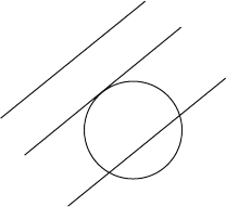
3.6.1.5. Theorem. Let C be a nondegenerate conic in P

. Any line L in P

intersects

C in 0, 1, or 2 points. Given any point p on C, there is one and only one line that inter-

sects C in that single point.

Proof. This fact is easily checked if C is a circle. See Figure 3.22. The general case

follows from the fact that any nonempty nondegenerate conic is projectively equiva-

lent to a circle.

Deﬁnition. If a line L meets a nondegenerate conic C in a single point p, then L is

called the tangent line to C at p. This deﬁnition applies to both the afﬁne and projec-

tive conics.

3.6.1.6. Theorem. If a nondegenerate conic is deﬁned in homogeneous coordinates

by the equation

then, in terms of homogeneous coordinates, the equation of the tangent line L to the

conic at a point P

(3.68)

In particular, [L] = [p

Q].

Proof. The line deﬁned by equation (3.68) clearly contains [p

]. It therefore sufﬁces

to show that if another point satisﬁed equation (3.68), then the conic would be degen-

erate. See [PenP86].

3.6.1.7. Corollary. The equation of the tangent line at a point (x

) of a conic

deﬁned by equation (3.35) is

Proof. Obvious.

ax hy f x hx by g y fx gy c

00 00 00

0++

()

+++

()

++ +=.

ppQ

0= .

ppQ

= 0,

184 3 Projective Geometry

Figure 3.22. Possible line/circle intersections.

We now describe solutions to ﬁve conic design problems in the plane R

. The fact

that the solutions are indeed correct follows easily from the above, in particular by

repeated use of Lemma 3.6.1.4. See [PenP86] for details.

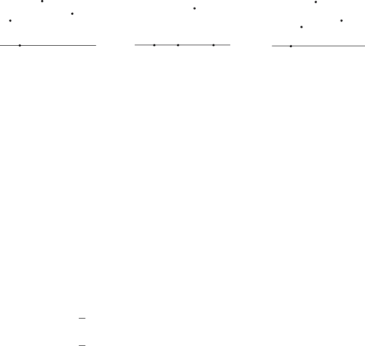
Conic design problem 1: To ﬁnd the equation of the conic passing through

four points p

, p

, and p

that has a given line L through one of these points

as tangent line. Assume that at least two of the points do not lie on L. If three points

lie off L, then no two of them are allowed to be collinear with the fourth. See Figure

3.23.

Solution. Assume that L is the tangent line at p

and that p

and p

do not lie on

L. Let L

be the line through p

and p

, let L

be the line through p

and p

, and let

be the line through p

and p

. Let [L] = [a,b,c] and [L

] = [a

]. Deﬁne symmetric

3 ¥ 3 matrices Q

and Q

Let C

(x,y) = 0 be the quadratic equation associated to Q

. Let p

= (x

). If

then there is a unique l so that C

) = 0 and that is the equation of the conic we

want.

3.6.1.8. Example. To ﬁnd the conic that passes through the points p

, p

= (2,-2),

= (2,2), p

= (5,0), and that has tangent line L at p

for the case where p

and L

have the values

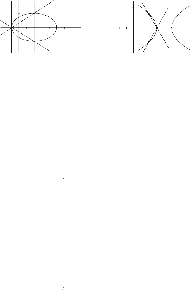
Solution for (a): See Figure 3.24(a). We have the following equations for the lines

ax bx

()

pL pL

10 1 0 30 3 0,, : ,, :

Cxy Cxy Cxy

ll,, ,,

()

()()

Q a b c a b c a b c a b c and

Qabcabcabcabc

144444

2222333333222

()( )

()()

()

()()

()

,, ,, ,, ,,

,, ,, ,, ,, .

3.6 Conic Sections 185

(a) Valid case

(b) Disallowed case

Figure 3.23. Conic design problem 1.

Therefore,

Solving C

(5,0) = 0 for l gives l=8/7, so that our conic is the ellipse

Solution for (b): See Figure 3.24(b). We have the following equations for the lines

This time

Solving C

(5,0) = 0 for l gives l=8/5, so that our conic is the hyperbola

Conic design problem 2: To ﬁnd the equation of the conic passing through three

points p

, p

, and p

that has two given lines L

and L

through two of these points

as tangent lines. Assume that the three points are not collinear and that the intersec-

Cxy x y

443 40,.

()

=- -

()

++=

Cxy x x xy xy

ll,.

()

3212 62 6

20:x-=

260:xy--=

260:xy+-=

Cxy x y

429 360,.

()

+-=

Cxy x x x y x y

ll,.

()

1 21 232232

20:x-=

2320:x y-+=

2320:x y++=

186 3 Projective Geometry

(a)

(b)

Figure 3.24. The conics that solve Example 3.6.1.6.

tion of the two lines is neither of the points where L

and L

are tangent to the conic.

See Figure 3.25.

Solution. Assume that L

and L

are tangent lines at p

and p

, respectively. Let L

be the line through p

and p

and let [L

] = [a

]. Deﬁne symmetric 3 ¥ 3 matrices

and Q

Let C

(x,y) = 0 be the quadratic equation associated to Q

. Let p

= (x

). If

then there is a unique l so that C

) = 0 and that is the equation of the conic we

want. Equivalently, if

then there is unique l so that (x

,1)Q

,1) = 0.

3.6.1.9. Example. To ﬁnd the conic that passes through the points p

= (4,-4) and

= (4,4), has tangent lines

at those points, and also passes through the point

Solution. First note that the line L

through p

and p

is clearly deﬁned by

40:x-=

abc

()

() ()

()

333

ppp00 10 10,, ,

240:,xy++=

240:,xy-+=

QQ Q

ll=+-

()

Cxy Cxy Cxy

ll,, ,,

()

()()

Q abc abc abc abc and Q abc abc

TT T

1 111 222 222 111 2 333 333

()( )

()()

()

()()

,, ,, ,, ,, ,, ,,.

3.6 Conic Sections 187

(a) Valid case

(b) Disallowed case (c) Disallowed case

Figure 3.25. Conic design problem 2.

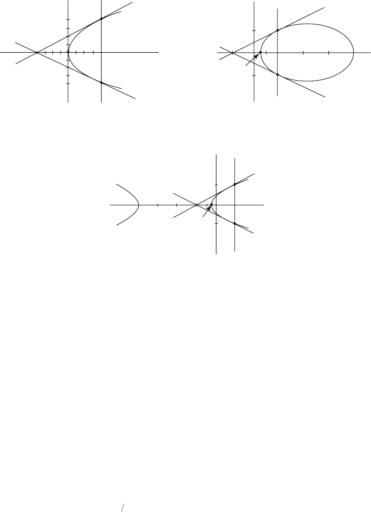
and

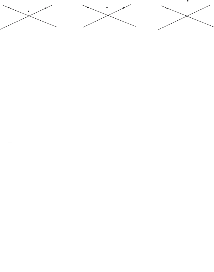
Case p

= (0,0): See Figure 3.26(a). The equation C

(0,0) = 0 leads to the impos-

sible condition l = 0. This corresponds to the case l=•. Therefore, the conic we are

looking for is the parabola

Case p

= (1,0): See Figure 3.26(b). The equation C

(1,0) = 0 leads to the solu-

tion l=-9/16. This time our conic is the ellipse

Case p

= (-1,0): See Figure 3.26(c). The equation C

(-1,0) = 0 leads to the solu-

tion l=25/16. This time our conic is the hyperbola

Cxyx xy

()

=-++=

916

4 68 9 64 0,.

Cxy x y x y x y x

•

()

=-+

()

=-,.24 24 4 4

Cxy x y x y x

ll,.

()

=-+

()

24 241 4

188 3 Projective Geometry

(a)

(b)

(c)

(0,0)

(1,0)

(–1,0)

(4,4)

(4,–4)

(4,4)

(4,–4)

Figure 3.26. The conics that solve Example 3.6.1.7.

Agoston M.K. Computer Graphics and Geometric Modelling: Mathematics

Подождите немного. Документ загружается.