Accardi L., Freudenberg W., Obya M. (Eds.) Quantum Bio-informatics IV: From Quantum Information to Bio-informatics

160

[7)(n)

(Bd,

...

,7)(n)

(Bm)] converges in

distribution

( i.e., weakly convergence

of

the

probability

distribution)

to

the

random

vector

[7)(B

1

),

. . . ,

7)(Bm)].

3.

A

Special

Type

of

a

Stochastic

Partial

Differential

Equation

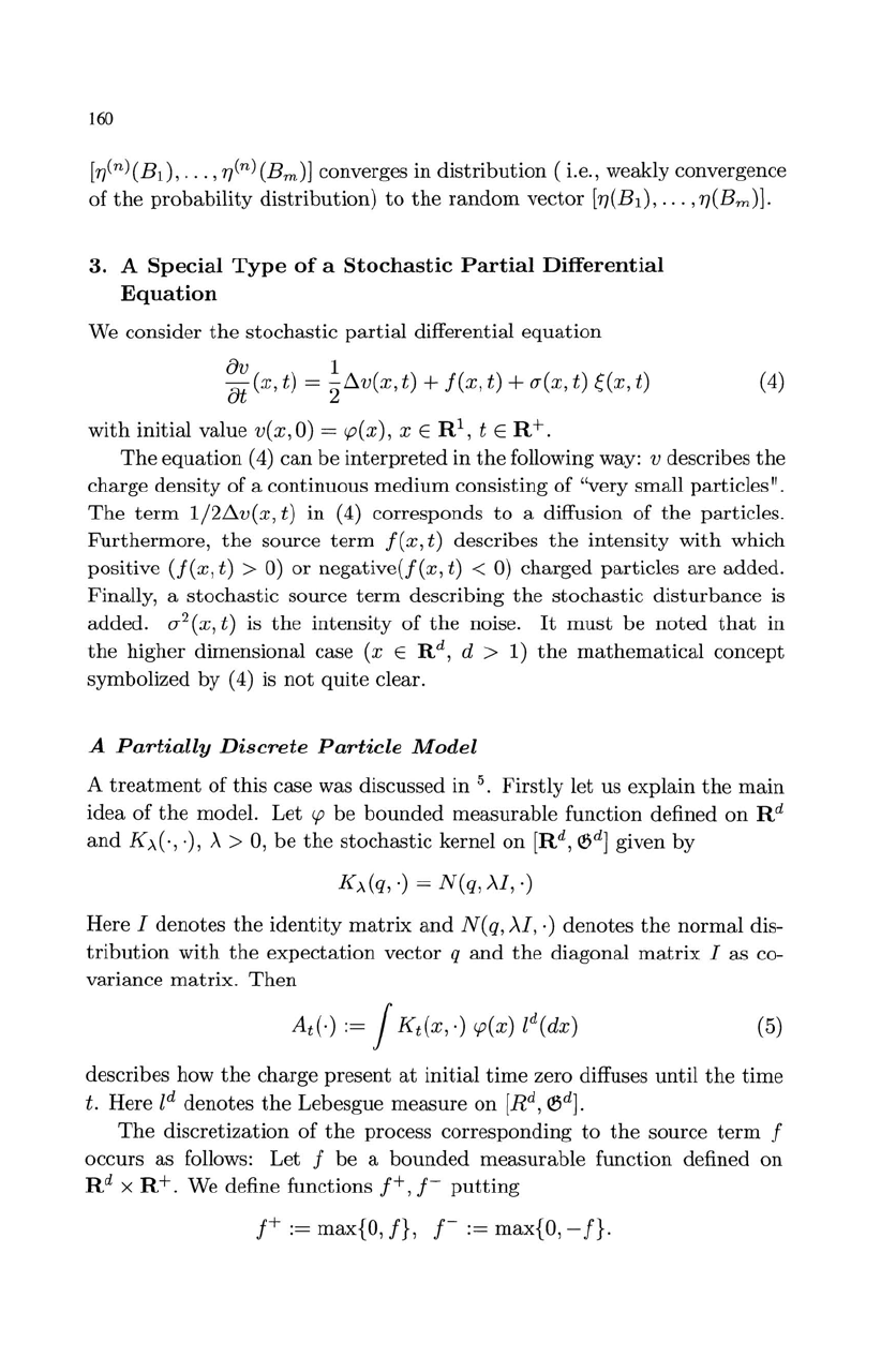
We consider

the

stochastic

partial

differential

equation

av

1

at

(x, t) =

2~v(x,

t) +

f(x,

t) +

(J"(x,

t)

~(x,

t)

with

initial value v(x,O) =

<p(x),

x E

Rl,

t E

R+.

(4)

The

equation

(4)

can

be

interpreted

in

the

following way: v describes

the

charge density of a continuous

medium

consisting

of

"very small particles".

The

term

1/2~v(x,

t)

in

(4) corresponds

to

a diffusion

of

the

particles.

Furthermore,

the

source

term

f(x,

t) describes

the

intensity

with

which

positive

(f(x,

t) > 0)

or

negative(f(x,

t) < 0) charged particles

are

added.

Finally, a

stochastic

source

term

describing

the

stochastic

disturbance

is

added.

(J"2(x,

t) is

the

intensity

of

the

noise.

It

must

be

noted

that

in

the

higher dimensional case (x E R

d,

d >

1)

the

mathematical

concept

symbolized by (4) is

not

quite

clear.

A

Partially

Discrete

Particle

Model

A

treatment

of

this

case was discussed

in

5.

Firstly

let us explain

the

main

idea

of

the

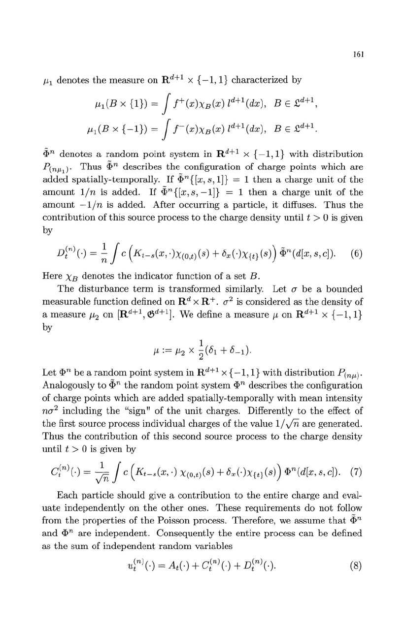
model. Let

<p

be

bounded

measurable function defined

on

R d

and

K)..(·,

.), ,\ >

0,

be

the

stochastic

kernel

on

[Rd,

Qjd] given by

K)..(q,·) = N(q,)..1,·)

Here I denotes

the

identity

matrix

and

N(q, ),,1,') denotes

the

normal

dis-

tribution

with

the

expectation

vector q

and

the

diagonal

matrix

I as co-

variance

matrix.

Then

(5)

describes how

the

charge present

at

initial

time

zero diffuses until

the

time

t.

Here

Zd

denotes

the

Lebesgue measure

on

[Rd,

Qjd].

The

discretization of

the

process corresponding

to

the

source

term

f

occurs as follows: Let f

be

a

bounded

measurable

function defined

on

R d X R

+.

We define functions f+, f -

putting

f+

:=

max{O,

f},

f-:=

max{O, -

f}

.

f-L1

denotes

the

measure

on

R

d

+

1

X {

-1,1}

characterized

by

f-L1(B

x {I}) = J

j+(XhB(X)

Zd+1(dx),

BE

£d+1,

f-L1(B

x

{-I})

= J

j-(X)XB(x)

Zd+l(dx),

BE

£d+1.

161

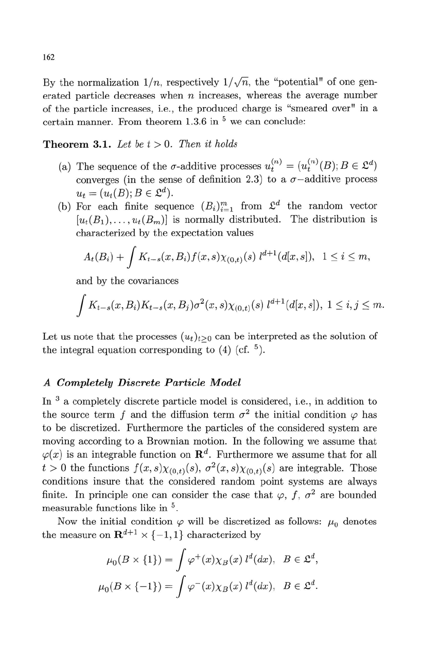
(j?n

denotes

a

random

point

system

in

Rd+1

x

{-I,

I}

with

distribution

P(nJ.Ll)'

Thus

(j?n

describes the_ configuration

of

charge

points

which

are

added

spatially-temporally.

If

{(In{[x,

S,

I])

= 1

then

a charge

unit

of

the

amount

l/n

is added.

If

(j?n{[x,

s,

-I])

= 1

then

a charge

unit

of

the

amount

-1/ n is added.

After

occurring

a particle,

it

diffuses.

Thus

the

contribution

of

this

source process

to

the

charge

density

until

t > 0 is given

by

D~n)O

=

~

J C

(Kt-s(x,

')X(O,t)(s) +

8xOX{t}(s))

(j?n(d[x,

s,

c]).

(6)

Here

XB

denotes

the

indicator

function

of

a

set

B.

The

disturbance

term

is

transformed

similarly.

Let

IJ

be

a

bounded

measurable

function defined

on

R d X R

+.

1J2 is considered as

the

density

of

a

measure

f-L2

on

[Rd+l,

Qjd+1].

We define a

measure

f-L

on

Rd+1

x

{-I,

I}

by

1

f-L

: =

f-L2

x

2"

(8

1

+ L

d·

Let

{(In

be

a

random

point

system

in

R

d+1

X {

-1,

I}

with

distribution

p(nJ.L)'

Analogously

to

(j?n

the

random

point

system

{(In describes

the

configuration

of

charge

points

which

are

added

spatially-temporally

with

mean

intensity

nIJ

2

including

the

"sign"

of

the

unit

charges. Differently

to

the

effect

of

the

first source process individual charges

of

the

value

1/

Vn

are

generated.

Thus

the

contribution

of

this

second source process

to

the

charge

density

until

t > 0 is given

by

c;n)

0 =

In

J c

(Kt-s(x,.)

X(O,t)(s)

+

8xOX{t}(s))

{(In (d[x,

s,

c]).

(7)

Each

particle

should

give a

contribution

to

the

entire

charge

and

eval-

uate

independently

on

the

other

ones.

These

requirements

do

not

follow

from

the

properties

of

the

Poisson process. Therefore, we

assume

that

(j?n

and

{(In

are

independent.

Consequently

the

entire

process

can

be

defined

as

the

sum

of

independent

random

variables

(8)

162

By

the

normalization lin, respectively

lifo,

the

"potential"

of one gen-

erated

particle decreases when n increases, whereas

the

average

number

of

the

particle increases, i.e.,

the

produced

charge is "smeared over"

in

a

certain

manner.

From

theorem

1.3.6 in 5

we

can

conclude:

Theorem

3.1.

Let

be

t >

O.

Then

it

holds

(a)

The

sequence

of

the

(J"-additive processes

u~n)

=

(u~n)

(B); B E £d)

converges (in

the

sense

of

definition 2.3)

to

a (J"-additive process

Ut

= (ut(B);

BE

£d).

(b) For each finite sequence

(Bi)'~l

from £d

the

random

vector

[ut(BI),

...

, ut(Bm)] is normally

distributed.

The

distribution

is

characterized by

the

expectation

values

and

by

the

covariances

Let

us

note

that

the

processes

(Ut)t>o

can

be

interpreted

as

the

solution

of

the

integral

equation

corresponding

to

(4) (cf.

5).

A

Completely

Discrete

Particle

Model

In

3 a completely discrete particle model is considered, i.e.,

in

addition

to

the

source

term

j

and

the

diffusion

term

(J"2

th

e initial condition

cp

has

to

be

discretized.

Furthermore

the

particles

of

the

considered

system

are

moving according

to

a Brownian motion.

In

the

following we assume

that

cp(x)

is

an

integrable function

on

Rd.

Furthermore

we assume

that

for all

t > 0

the

functions j(x,s)x(O,t)(s), (J"2(x,s)X(0,t)(s)

are

integrable.

Those

conditions insure

that

the

considered

random

point

systems

are

always

finite.

In

principle one

can

consider

the

case

that

cp,

j,

(J"2

are

bounded

measurable

functions like in

5.

Now

the

initial condition

cp

will

be

discretized as follows:

/-to

denotes

the

measure

on

R d+ 1 X

{-1,

I}

characterized by

/-to(B

x {I}) = J

cp+

(X)xB (x) ld(dx),

BE

£d,

/-to(B

x

{-I})

= J

CP

- (X)XB(X) ld(dx),

BE

£d.

163

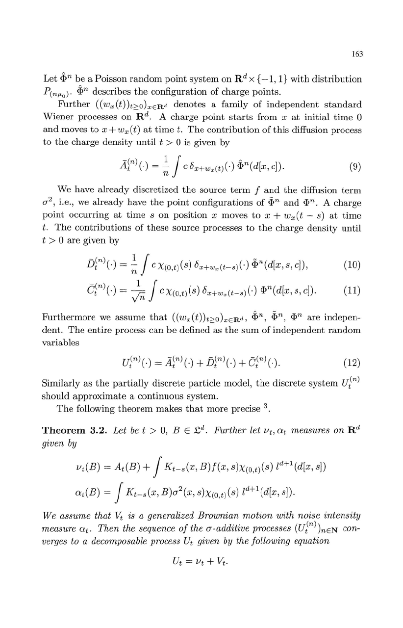
Let

~n

be

a Poisson

random

point

system

on

R d X {

-1,

I}

with

distribution

p(nl-'o)'

~n

describes

the

configuration

of

charge points.

Further

((wx(t))t>O)xERd

denotes

a family

of

independent

standard

Wiener

processes on Rd. A charge

point

starts

from x

at

initial

time

0

and

moves

to

x + wx(t)

at

time

t.

The

contribution

of

this

diffusion process

to

the

charge

density

until t > 0 is given

by

(9)

We have

already

discretized

the

source

term

f

and

the

diffusion

term

J2, i.e., we

already

have

the

point

configurations

of

~n

and

q,n. A charge

point

occurring

at

time

s

on

position

x moves

to

x +

Wx

(t - s)

at

time

t.

The

contributions

of

these

source processes

to

the

charge density

until

t > 0

are

given

by

-en)

11

-

D

t

(-)

=;

c X(O,t)(s) Dx+wx(t-s)(-) q,n(d[x,

s,

c]),

(10)

c;n)(-)

=

In

1 C

X(O,t)(S)

Dx+wx(t-s)(-) q,n(d[x,

s,

c]).

(11)

Furthermore

we

assume

that

((w

x

(t))t2:0)XERd,

~n,

q,n

are

indepen-

dent.

The

entire

process

can

be

defined as

the

sum

of

independent

random

variables

(12)

Similarly

as

the

partially

discrete

particle

model,

the

discrete

system

Ut(n)

should

approximate

a continuous system.

The

following

theorem

makes

that

more

precise

3.

Theorem

3.2.

Let

be

t >

0,

B E £d. Further let Vb

at

measures on Rd

given

by

Vt(B)

=

At(B)

+ 1

Kt-s(x,

B)f(x,

S)x(O,t)(S) ld+l(d[x,

s])

at(B)

= 1

Kt-s(x,

B)J

2

(x, S)x(O,t)(S)

1d+1(d[x, s]).

We assume that

"\it

is a generalized Brownian

motion

with noise

intensity

measure

at.

Then the sequence

of

the J-additive processes (Ut(n))nEN con-

verges to a decomposable process U

t

given

by

the following equation

164

Remark

3.1.

This

theorem

means

that

the

completely discrete particle

model

approximates

a continuous

system

being different from

the

limit

considered

in

5,

i.e.,

the

limit

of

the

completely discrete model

has

the

same

expectation

values

but

different covariances,

compared

with

the

limit

considered in

5.

4.

Some

Lemmas

For

the

proof

of

the

main

theorem

in 3 (theorem 3.2

in

this

paper)

it

is

necessary

to

use

the

following lemmas.

Lemma

4.1.

Let

\[Tn

be

a Poisson random point

system

with

intensity

measure

nf.1

where

f.1

is a locally finite measure on G

and

n E

N.

u(n)

denotes the CT-additive process defined by

u(n)

:=

~

\[Tn.

Then

the sequence

(u(n)

)nEN

converges to the (trivial) CT-additive process

f.1,

i. e.,

AUCn)

(g)

-+

exp{ifg(x)f.1(dx)}

(n-++oo).

Lemma

4.2.

Let

<pr,<p~

be

independent Poisson random

point

systems

with

intensity

measure

nf.1

where

f.1

is a locally finite measure on G

and n

E

N.

u(n)

denotes the CT-additive process defined by

u(n)

:=

vk(<p

1

-

<p~).

Then

the sequence

(u(n))nEN

converges to a generalized

Brownian

motion

U with noise

intensity

measure

f.1,

i.e.,

AUCn)

(g)

--+

exp

[-~

f{g(X)}2f.1(dx)]

(n

-+

+00).

Now let

kt(x

, y)

be

the

density

of

the

transition

probability

of

the

d-

dimensional

standard

Wiener

process, i.e.,

d

kt(x,y)

=

(_1_)"2

exp

(-~llx

_

Y112)

(t>

Q,x,y

E R

d

).

27rt

2t

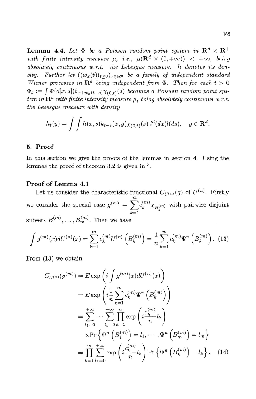
Lemma

4.3.

Let

<P

be

a

Poisson

random point

system

in

R d with finite in-

tensity

measure

f.1

being absolutely continuous

w.

r.

t.

the Lebesgue measure.

h denotes its density. Further let

((w

x

(t))t20)XERd

be

a family

of

indepen-

dent standard

Wiener

processes

in

R d being independent

from

<P.

Then

for

each t > Q

<P

t

:=

f

<P(dx)

Dx+wx(t)

becomes a Poisson random point

system

in

R d with finite

intensity

measure

f.1t

being absolutely continuous

w.

r.

t.

the

Lebesgue measure with density

165

Lemma

4.4.

Let

1>

be

a Poisson random

point

system

in

Rd

x

R+

with finite

intensity

measure

f-L,

i.e.,

f-L(R

d

x (0,

+(0))

< +00, being

absolutely continuous

w.

r.

t.

the Lebesgue measure. h denotes its den-

sity. Further let

((wx(t))t:"O)xERd

be

a

family

of

independent

standard

Wiener

processes

in

Rd

being independent

from

1>.

Then

for

each t > 0

1>t

:=

J

1>(d[x,

s])Ox+wx(t-s)X(O,t)(s) becomes a Poisson

random

point sys-

tem

in

R d with finite

intensity

measure

f-Lt

being absolutely continuous

w.

r.

t.

the Lebesgue measure with density

5.

Proof

In

this

section we give

the

proofs

of

the

lemmas

in

section 4. Using

the

lemmas

the

proof

of

theorem

3.2 is given in

3.

Proof

of

Lemma

4.1

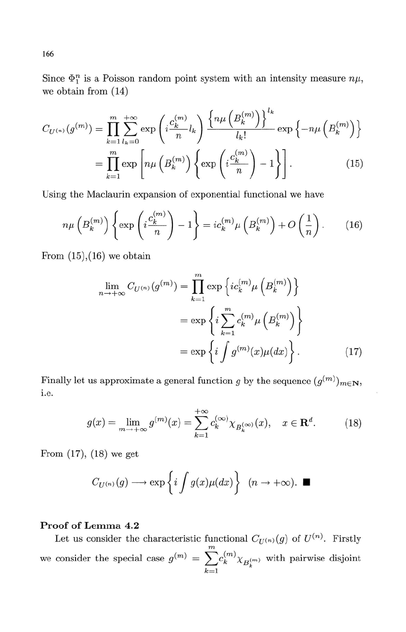
Let

us consider

the

characteristic

functional Cu(n)

(g)

of

u(n).

Firstly

m

we consider

the

special case

gem)

=

Lc~m)XB("')

with

pairwise disjoint

k

k=l

subsets

Bi

m

),

...

,

B~m).

Then

we

have

J gCm)(x)du(n)(x) =

fc~m)u(n)

(Bk

m

)) =

~

fc~m)wn

(Bk

m

)).

(13)

k=l

From

(13)

we

obtain

Cu(n)

(g(m))

=

Eexp

(i

J

g(m)

(x)du(n)

(x))

=

Eexp

(i~

~c~m)wn

(Bk

m

)))

+00 +00

m

((m))

= L

...

L

II

exp

iC~

lk

h=O

lk=O

k=l

xPr{wn(Bim))

=h,'"

,Wn(B~m))

=lm}

=

fL~

exp

(iC~)

lk)

Pr

{w

n

(Bk

m

)) =

lk}'

(14)

166

Since

<D1

is a Poisson

random

point

system

with

an

intensity

measure

nj.L,

we

obtain

from (14)

Using

the

Maclaurin

expansion

of

exponential

functional

we have

From

(15),(16) we

obtain

=exp{i~c~m)j.L(Bkm))

}

=

exp

{i

J

g(m)

(x)j.L(dx)

}.

(17)

Finally

let

us

approximate

a

general

function

g

by

the

sequence

(g(m))mEN,

i.e.

From

(17), (18) we

get

CU(n)

(g)

~

exp

{i

J g(X)j.L(dX)}

(n

--+

+00)

.•

Proof

of

Lemma

4.2

Let

us consider

the

characteristic

functional

Cu(n)

(g)

of

u(n).

Firstly

m

we consider

the

special case

gem)

=

Lc~m)XB(=)

with

pairwise disjoint

k

k=l

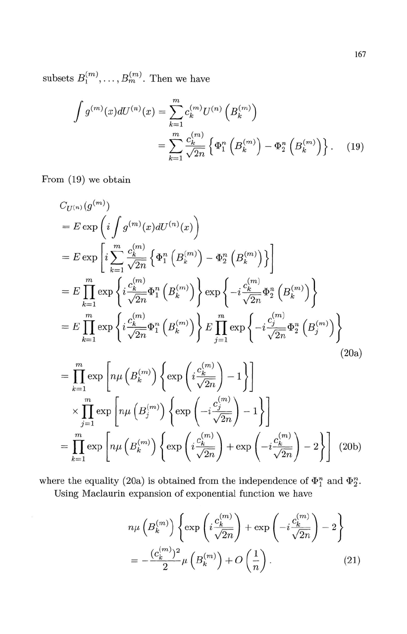
167

subsets

Bi

m

),

...

,

B~m).

Then

we have

J

g(m)

(x)du(n) (x) = f

ckm)u

(n)

(Bk

m

))

k=l

m

(m)

=

~

{<1>7

(Bk

m

))

-

<1>~

(Bkm))}.

(19)

From (19) we

obtain

=

IT

exp

[n~

(Bk

m

))

{ex

p

«~)

-I}]

x n

eX+M

(Bjm))

{ex

p

(

-i$;

)

I}]

=

IT

exp

[n~(Bkm))

{ex

p

«~)

+exp

(-ij;)

-2}]

(20b)

where

the

equality (20a) is

obtained

from

the

independence of

<1>f

and

<1>2.

Using Maclaurin expansion of exponential function we have

n~

(Bk

m

))

{ex

p

(ij;)

+exp

(-ij;)

-

2}

= _

(C

k

:))2

~

(Bk

m

))

+ 0

(~).

(21)

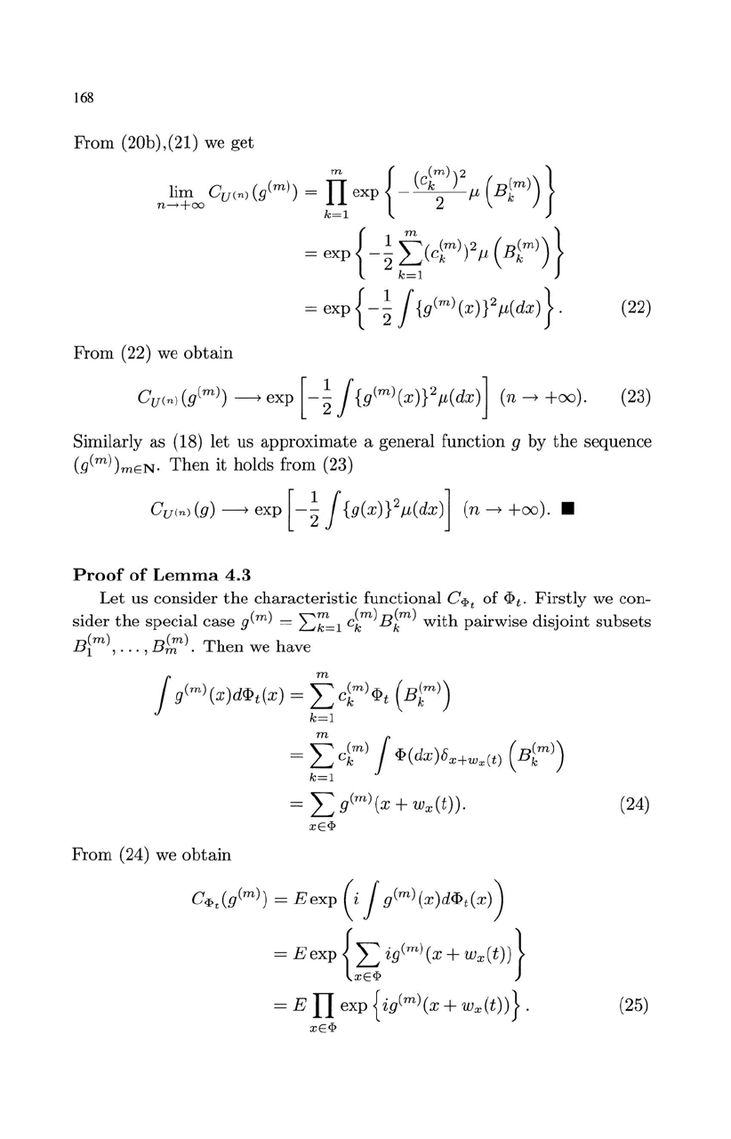
168

From

(20b),(21) we

get

From

(22)

we

obtain

Gu(n)

(g(rn))

-----+

exp

[-~

J {g(rnl(x)}2

fL

(dX)]

(n

----+

+00). (23)

Similarly as (18) let us

approximate

a general function g by

the

sequence

(g(rn)

)rnEN.

Then

it

holds from (23)

Gu(n)

(g)

-----+

exp

[-~

J {g(X)}2

fL

(dX)]

(n

----+

+00)

.•

Proof

of

Lemma

4.3

Let

us

consider

the

characteristic functional

Gt

of

t.

Firstly

we con-

sider

the

special case

g(rn)

=

EZ'=l

c~rn)

Bk

rn

)

with

pairwise disjoint

subsets

B

(rn)

B(rn)

Th

h

1 ,

...

,

rn·

en

we

ave

J

g(rn)

(x)dt(x)

=

f>~m)t

(Bk

m

))

k=l

=

f>~m)

J

(dx)8

x

+

wx

(t)

(Bk

m

))

k=l

= L g(m)(x + wx(t)).

(24)

xE

From

(24) we

obtain

Gt(g(m))

=

Eexp

(i

J

g(m)

(X)dt(X))

=

EexP{Lig(ml(X+wx(t))}

xE

= E

II

exp

{ig(m)(X +

Wx(t))}.

(25)

xE

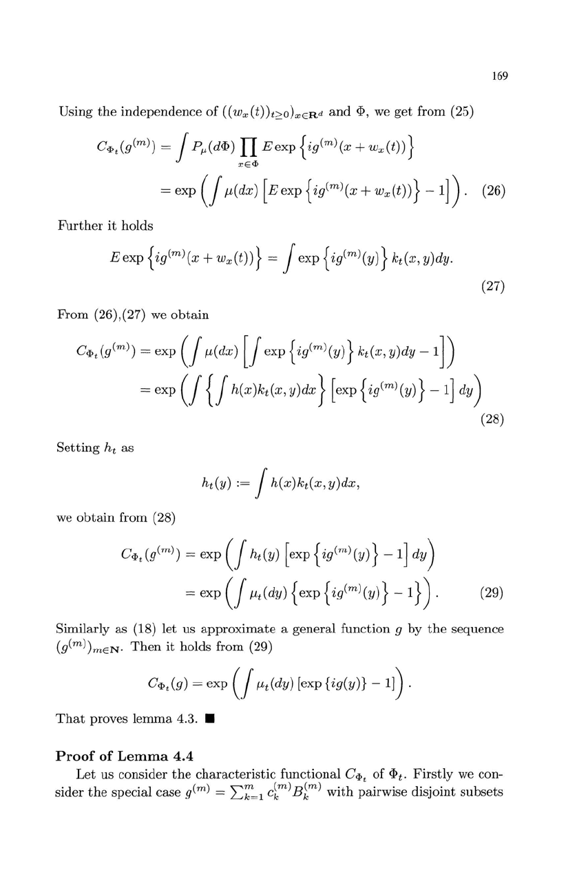
Using

the

independence

of

((wx(t)k~O)xERd

and

<P,

we

get

from (25)

G'Pt(g(m»)

= J

PJ-L(d<p)

II

Eexp

{i9(m)(X

+wx(t))}

xE'P

169

=

exp

(J

J-l(dx)

[Eexp{ig(m)(x+wx(t))}

-1]).

(26)

Further

it

holds

E exp {ig(m)(x + Wx(t))} = J

exp

{ig(m)(y)} kt(x, y)dy.

(27)

From

(26),(27) we

obtain

G'Pt(g(m»)

= exp

(J

J-l(dx)

[J

exp

{ig(m)(y)}

kt(x,y)dy

-1])

=

exp

(J

{J

h(x)kt(x, Y)dX} [ex

p

{i9(m)(y)} -

1]

d

Y

)

(28)

Setting

h

t

as

ht(y)

:=

J h(x)kt(x, y)dx,

we

obtain

from (28)

G'P

t

(g(m»)

=

exp

(J

ht(y) [ex

p

{i9(m)(y)}

-1]

d

Y

)

= exp

(J

J-lt(dy)

{ex

p

{i9(m)(y)} -I}) . (29)

Similarly as (18) let

us

approximate

a general function 9 by

the

sequence

(g(m»)mEN.

Then

it

holds from (29)

G'Pt(g)

= exp

(J

J-lt(dy)

[exp{ig(y)}

-IJ).

That

proves

lemma

4.3

.•

Proof

of

Lemma

4.4

Let

us consider

the

characteristic functional

G'P

t

of

<Pt.

Firstly

we con-

sider

the

special case

g(m

) =

2::;;'=1

ci

m

)

Bk

m

)

with

pairwise disjoint

subsets

Accardi L., Freudenberg W., Obya M. (Eds.) Quantum Bio-informatics IV: From Quantum Information to Bio-informatics

Подождите немного. Документ загружается.