Ablowitz M.A. Nonlinear Dispersive Waves: Asymptotic Analysis and Solitons
Подождите немного. Документ загружается.


4.4 Method of multiple scales: Nonlinear example 85
The leading-order equation and solution are the same as in the previous
example,
y
0
(t, T) = A(T )e
it
+ c.c.
The next-order equation is
O(ε): y
1,tt
+ y
1
= −2y
0,tT
− y
3
0
.
Substituting the leading-order solution in the right-hand side and expanding
the nonlinear term leads to
y
1,tt
+ y
1
= −(2iA
T
e
it
+ c.c.) + (Ae
it
+ A
∗
e
−it
)
3
= −(2iA
T
e
it
+ c.c.) + (A
3
e
3it
+ 3A
2
A
∗
e
it
+ c.c.)
= −(2iA
T
− 3|A|
2
A)e
it
6789
secular
+ A
3
e
3it
6789
non-secular
+ c.c.
It is important to distinguish the terms that multiply e
it
from those that multiply
e
3it
, because the former is a secular term, i.e., it satisfies the homogeneous
solution for y
1
, whereas the second one does not. Therefore, we must remove
the secular terms, which multiply e
it
, but keep the non-secular terms, which
multiply e
3it
, in the equation for y
1
– the non-secular term results in a bounded
contribution to y
1
. To remove secularity, we require that
2iA
T
= 3|A|
2
A (4.17)
and the equation for y
1
becomes
y
1,tt
+ y
1
= A
3
e
3it
+ c.c. (4.18)
The solution of the (complex-valued) ODE (4.17) can be found by noting that
|A|
2
is a conserved quantity in time. One way to see this is by multiplying (4.17)
by A
∗
, subtracting the complex conjugate, and integrating:
2iA
T
A
∗
+ 2iA
∗
T
A = 3|A|
2
AA
∗
− 3|A|
2
A
∗
A
and therefore i(|A|
2
)
T
= 0. Hence |A|
2
(T ) = |A|
2
(0) = |A
0
|
2
, where A
0
is our
arbitrary constant. Using this conservation relation we can rewrite (4.17)as
2iA
T
= 3|A
0
|
2
A.
This is now a linear equation for A and its solution is given by
A(T ) = A
0
e
−
3i
2
|A
0
|
2
T
= A
0
e
−
3i
2
|A
0
|
2
εt
.

86 Perturbation analysis
Note A(T ) depends on T = εt, so we can assume that A(T) is constant when
integrating the equation for y
1
in (4.18). Assuming that y
1
= Be
3it
+ c.c. gives
B = −A
3
/8, which is bounded, and therefore
y
1
(t) = −
1
8
A
3
(T )e
3it
+ c.c. + O(ε) = −
1
8
A
3
0
e
−
9i
2
|A
0
|
2
εt
e
3it
+ c.c. + O(ε).
Finally, the perturbed solution we find is
y(t) = A
0
e
(
1−
3ε
2
|A
0
|
2
)
it
+ εy
1
(t) + c.c.,
= A
0
e
(
1−
3ε
2
|A
0
|
2
)
it
−
ε
8
A
3
0
e
−
9i
2
|A
0
|
2
εt
e
3it
+ c.c.
Inspecting our solution we note that the second term (the one multiplied by
ε) plays a minor role compared with the first term, since the amplitude of the
second term is bounded and so remains O(ε) small relative to the first term for
all values of t. We therefore focus our attention on the first term: its effective
frequency is given by
Ω=1 −
3ε
2
|A
0
|
2
. (4.19)
Therefore, when ε>0, the additional frequency contribution decreases with
amplitude |A
0
| (beyond the linear solution) and the period of oscillations
increases (since T = 2π/Ω). This is sometimes called a “soft spring”, in anal-
ogy with a spring whose period is elongated compared with a linear spring.
Conversely, when ε<0 the frequency increases and the period of oscillations
decreases. This is called a “hard spring”.
Since the equation is conservative and there is only a (nonlinear) frequency
shift, this problem can also be done by the frequency-shift method. This is left
as an exercise.
4.5 Method of multiple scales: Linear and nonlinear
pendulum
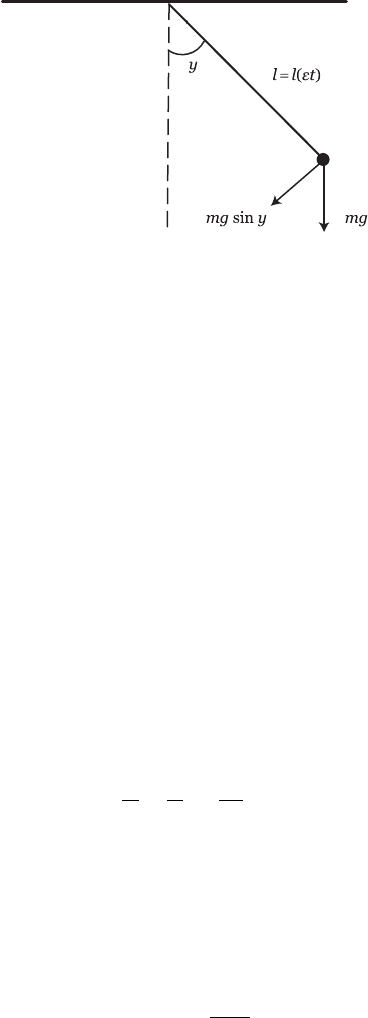
For our final application of multiple scales to ODEs, we will look at a nonlinear
pendulum with a slowly varying length; see Figure 4.1. Newton’s second law
of motion gives
ml¨y + mg sin(y) = 0
as the equation of motion, where m is the pendulum mass, g the gravitational
constant of acceleration, and l the slowly varying length. This implies that
¨y + ρ
2
(εt)sin(y) = 0, (4.20)
4.5 Method of multiple scales: Linear and nonlinear pendulum 87
Figure 4.1 Nonlinear pendulum.
where for convenience we denote ρ
2
(εt) ≡ g/l(εt), or more simply ρ
2
(T ) with
T ≡ εt, which we assume is smooth. If the length were constant, an exact
solution would be available in terms of elliptic functions.
Associated with this pendulum is what is usually called an adiabatic invari-
ant, i.e., a quantity in the system that is asymptotically invariant when a system
parameter is slowly (adiabatically) changed. While analyzing the pendulum
problem, we will look for adiabatic invariants. Adiabatic invariants received
much attention during the development of the theory of quantum mechanics,
cf. Goldstein (1980) and Landau and Lifshitz (1981), and more recently in such
areas as plasma physics, particle accelerators, and galactic dynamics, etc.
4.5.1 Linear pendulum
To start, we will consider the linear problem
¨y + ρ
2
(εt)y = 0. (4.21)
Suppose we assume a “standard” multi-scale solution in the form y(t) =
y(t, T; ε). Expand d/dt and y as
d
dt
=
∂
∂t
+ ε
∂
∂T
,
y(t) = y
0
(t, T) + εy
1
(t, T) + ε
2
y
2
(t, T) + ···
and substitute them into (4.21). Collecting like powers of ε gives
O(1):
Ly
0
≡ ∂
2
t
y
0
+ ρ
2
(T )y
0
= 0.
O(ε):
Ly
1
= −2
∂
2
y
0
∂t∂T
.

88 Perturbation analysis
The leading-order solution is
y
0
= A(T)exp(iρt) + c.c.
Notice that
∂
T
y
0
= (A
T
+ itρ
T
)exp(iρt) + c.c.
grows as t →∞; i.e., it is secular! The problem is that we chose the wrong fast
time-scale. We modify the fast scale in y as follows:
y(t) = y(Θ(t), T; ε),
where Θ
t
= ω(εt) and ω will be chosen so that the leading-order solution is not
secular. Expand d/dt as
d
dt
=Θ
t
∂
∂Θ
+ ε
∂
∂T
= ω(T )
∂
∂Θ
+ ε
∂
∂T
.
A little care must be taken in calculating d
2
/dt
2
, since ω is a function of the
slow variable: we get
d
2
dt
2
=
ω(T )
∂
∂Θ
+ ε
∂
∂T
ω(T )
∂
∂Θ
+ ε
∂
∂T
= ω
2
∂
2
∂Θ
2
+ ε
2ω
∂
2
∂Θ∂T
+ ω
T
∂
∂Θ
+ ε
2
∂
2
∂T
2
. (4.22)
Substituting this into (4.21) and expanding y = y
0
+ εy
1
+ ··· we get the first
two equations
O(1):
ω
2
(T )
∂
2
y
0
∂Θ
2
+ ρ
2
(T )y
0
= 0.
O(ε):
ω
2
(T )
∂
2
y
1
∂Θ
2
+ ρ
2
(T )y
1
= −
ω
T
∂y
0
∂Θ
+ 2ω
∂
2
y
0
∂T ∂Θ
.
The leading-order solution is
y
0
= A(T)exp
i
ρ
ω
Θ
+ c.c.
To prevent secularity at this order we require that
∂y
0
∂T
= (A
T
+ i(ρ/ω)
T
θA)e
i(ρ/ω)θ
is bounded in θ. Hence we must take ω/ρ to be constant in order to remove
the secular term. The choice of constant does not affect the final result, so

4.5 Method of multiple scales: Linear and nonlinear pendulum 89
for convenience we take ω = ρ. The order ε equation then becomes, after
substituting in the expression for y
0
,
ρ
2
(T )
∂
2
y
1
∂Θ
2
+ y
1
= −
iρ
T
Ae
iΘ
+ 2iA
T
ρe
iΘ
+ c.c.
.
To remove secular terms, we require
2ρA
T
+ Aρ
T
= 0,
2ρA
∗
T
+ A
∗
ρ
T
= 0.
Multiplying the first equation by A
∗
, the second by A, and then adding, we find
that
∂
∂T
ρ|A|
2
= 0 ⇒ ρ(T )|A(T )|
2
= ρ(0)|A(0)|
2
=
E
ρ
,
where E = ρ
2
A
2
is related to the unperturbed energy E = ˙y
2
/2 + ρ
2
y
2
/2,
from (4.21); thus ρ(T )|A(T )|
2
= E/ρ is constant in time. This is usually called
the adiabatic invariant. Notice that ρ(T )|A(T )|
2
is constant on the same time-
scale as the length is being varied. Also, using separation of variables on the
equation for A
T
,
A
T
A
=
−ρ
T
2ρ
⇒ log(Aρ
1/2
) = constant ⇒ A(T ) =
C
ρ
1/2
(T )
where C is constant. Since ω = ρ,
Θ(t) =
t
0
ρ(εt
) dt
=
1
ε
εt
0
ρ(s) ds.
The leading-order solution is then
y(t) ∼
C
ρ(εt)
exp
$
i
ε
εt
0
ρ(s) ds
2
+ c.c.
Alternatively, we can arrive at the same approximate solution using the so-
called WKB method,
1
cf. Bender and Orszag (1999). Instead of introducing
multiple time-scales, let T = εt and simply change variables in (4.21) to get
ε
2
d
2
y
dT
2
+ ρ
2
(T )y(T ) = 0.
1
The WKB method is named after Wentzel, Kramers and Brillouin who used the method
extensively. However, these ideas were used by others including Jeffries and so is sometimes
referred to as the WKBJ method.
90 Perturbation analysis
If ρ were constant, the solution would be y = e
iρ/ε
+ c.c. This suggests that
we look for a solution in the form y ∼ e
iφ(T ;ε)/ε
+ c.c. Using this ansatz, we
find
−φ
2
T
+ iεφ
TT
+ ρ
2
= 0.
We now expand φ as φ = φ
0
+ εφ
1
+ ε
2
φ
2
+ ··· to get the leading-order
equation
∂φ
0
∂T
= ±ρ(T ) ⇒ φ
0
= ±
T
0
ρ(s) ds + μ
0
,
where μ
0
is the constant of integration. The O(ε) equation is −2φ
0T
φ
1T
+
iφ
0TT
= 0, so
∂φ
1
∂T
=
i
2
φ
0TT
φ
0T
=
i
2
∂
∂T
log |φ
0T
|,
which gives
φ
1
=
i
2
log |φ
0T
| =
i
2
log(ρ).
Thus, in terms of the original variables:
y(t) ∼ exp
%
i
(
φ
0
+ εφ
1
)
/ε
&
,
= exp
i
ε
εt
0
ρ(s) ds + μ
0
−
1
2
log(ρ(εt))
+ c.c.
Setting C = exp(iμ
0
/ε),
y(t) ∼
C
ρ(εt)
exp
i
ε
εt
0
ρ(s) ds
+ c.c.,
which is identical to the multiple-scales result.
4.5.2 Nonlinear pendulum
Now we will analyze the nonlinear equation, (4.20),
d
2
y
dt
2
+ ρ
2
(T )sin(y) = 0.
These and more general problems were analyzed by Kuzmak (1959), see also
Luke (1966). We will see that this problem is considerably more complicated
than the linear problem: multiple scales are required. As in the linear problem,
4.5 Method of multiple scales: Linear and nonlinear pendulum 91
assuming y = y(Θ, T ; ε) = y
0
+ εy
1
+ ···, T = εt and using (4.22) to expand
d
2
/dt
2
, the leading- and first-order equations are, respectively,
ω
2
y
0ΘΘ
+ ρ
2
sin(y
0
) = 0,
L(y
1
) = ω
2
y
1ΘΘ
+ ρ
2
cos(y
0
)y
1
= −
(
ω
T
y
0Θ
+ 2ωy
0ΘT
)
= F
1
.
The crucial part of the perturbation analysis is to understand the leading-order
equation. Multiplying the leading-order equation by y
0Θ
, we find the “energy
integral”:
∂
∂Θ
ω
2
2
y
2
0Θ
− ρ
2
cos(y
0
)
= 0 ⇒ (4.23a)
ω
2
2
y
2
0Θ
− ρ
2
cos(y
0
) = E(T ) ⇒ (4.23b)
ω
2
y
2
0Θ
= 2(E + ρ
2
cos(y
0
)). (4.23c)
Notice (i) that the coefficient ρ is constant with respect to Θ and so is E; (ii) the
left-hand side of the integral equation (4.23b) is not necessarily positive. If we
redefine
˜
E = E + ρ
2
so that ω
2
y
2
0Θ
/2 + ρ
2
(1 − cos y
0
) =
˜
E, then
˜
E ≥ 0 and
˜
E
is an energy. However, we use E to simplfy our notation. Solving for dy
0
/dΘ
and separating variables gives
dy
0
2
3
E + ρ
2
cos y
0
4
=
dΘ
ω
.
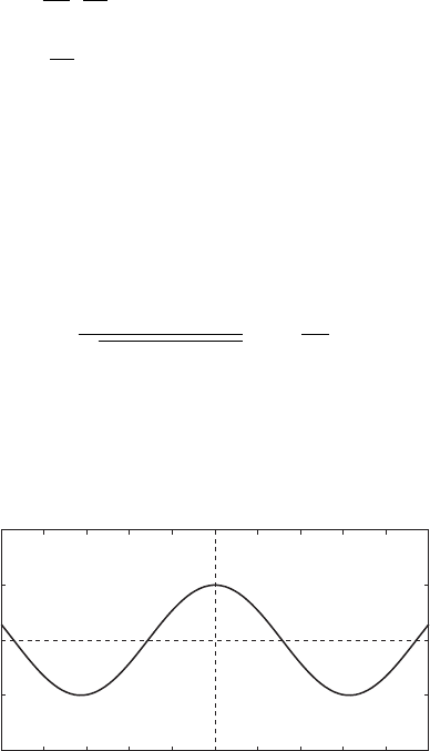
We will be concerned with periodic solutions in Θ; see also the phase plane in
Figure 4.2. Periodic solutions are obtained for values |y|≤y
∗
obtained from
cos y
∗
= −E/ρ
2
.
−5 0 5−4 −3 −2 −1 1 2 3 4
−2
−1
0
1
2
y
0
y
0
Θ
y
*
Figure 4.2 Phase plane.

92 Perturbation analysis
The period of motion, P,is
P = ω
5
dy
0
2
3
E + ρ
2
cos y
0
4
,
where the loop integral is taken over one period of motion. Since cos(y
0
)is
even and symmetric, we can also calculate the period from
P = 4ω
y
∗
0
dy
0
2
3
E + ρ
2
cos y
0
4
. (4.24)
Since the motion is periodic, for any integer n
y
0
(Θ+nP, T ) = y
0
(Θ, T ).
At this stage P is a function of T , thus
∂y
0
(Θ+nP, T )
∂T
= n
∂P
∂T
∂y
0
(Θ, T )
∂Θ
+
∂y
0
(Θ, T )
∂T
. (4.25)
For a well-ordered perturbation expansion, the first derivative
∂y
0
(Θ+nP, T )/∂T must be bounded. However, from (4.25), ∂y
0
(Θ+nP, T )/
∂T →∞as n →∞. We can eliminate this divergence if we set ∂P/∂T = 0,
i.e., we require the period to be constant. The choice of constant does not
affect the final result, so we can take P = 2π and then we have from (4.24),
ω = ω(E) =
π
2
y
∗
0
dy
0
2
3
E + ρ
2
cos y
0
4
. (4.26)
To find out how E varies, we must go to the next-order equation, namely,
Ly
1
=
ω
2
∂
2
Θ
+ ρ
2
(T ) cos(y
0
)
y
1
= F
1
= −
(
ω
T
y
0Θ
+ 2ωy
0ΘT
)
. (4.27)
We will not actually solve the O(ε) equation here, but instead we only need to
derive a so-called solvability condition using a Fredholm alternative. We start
by examining the homogeneous equation adjoint to (4.27): L
∗
W = 0, where L
∗
is the adjoint to the operator L, with respect to the inner product
Ly, W =
2π
0
(
Ly
)
WdΘ=y, L
∗
W;
integration by parts shows that L = L
∗
, i.e., the operator L is self-adjoint. Now
consider
Ly
1
=
ω
2
∂
2
Θ
+ ρ
2
(T ) cos(y
0
)
y
1
= F
1
,
L
∗
W = LW = 0,

4.5 Method of multiple scales: Linear and nonlinear pendulum 93
where W is the periodic solution of the adjoint equation. There is another, non-
periodic solution to the adjoint problem (obtained later for completeness); but
since we are only interested in periodic solutions, we do not need to consider
it in the secularity analysis. Multiply the first equation by W, the second by y
1
,
and subtract to find
ω
2
∂
∂Θ
(
Wy
1Θ
− W
Θ
y
1
)
= WF
1
.
Integrating this over one period and using the periodicity of the solution y
1
gives
2π
0
WF
1
dΘ=0 (4.28)
as a necessary condition for a periodic solution of the O(ε) equation to exist.
This orthogonality condition must hold for the periodic solution, W,ofthe
homogeneous problem, which we will now determine. Operate on the leading-
order equation with ∂/∂Θ to find
ω
2
y
0ΘΘΘ
+ ρ
2
cos(y
0
)y
0Θ
= 0,
i.e., y
0Θ
is a solution of LW = 0; hence we set W
1
= y
0Θ
. This is the periodic,
homogeneous solution. To find the non-periodic homogeneous solution operate
on the leading-order equation with ∂/∂E to find
Ly
0E
= ω
2
y
0EΘΘ
+ ρ
2
cos(y
0
)y
0E
= −(ω
2
)
E
y
0ΘΘ
.
On the other hand, for any constant α,
L(αΘy
0Θ
) = ω
2
∂
2
∂Θ
2
(
αΘy
0Θ
)
+ ρ
2
cos(y
0
)αΘy
0Θ
= α
2ω
2
y
0ΘΘ
+Θ
ω
2
y
0ΘΘΘ
+ ρ
2
cos(y
0
)y
0Θ
.
The term in parentheses vanishes and we have
L(αΘy
0Θ
) = 2αω
2
y
0ΘΘ
.
Hence for the combination, y
0E
+ αΘy
0Θ
:
L(y
0E
+ αΘy
0Θ
) = L(y
0E
) + L(αΘy
0Θ
)
= −
ω
2
E
y
0ΘΘ
+ 2αω
2
y
0ΘΘ
.
Thus, if we set α = ω
E
/ω,
L(y
0E
+ αΘy
0Θ
) = 0
94 Perturbation analysis
and we have the second solution:
W
2
= y
0E
+
ω
E
ω
Θy
0Θ
,
cf. Luke (1966). This solution, however, is not generally periodic since ω
E
0
in the nonlinear problem. We therefore need only one homogeneous solution
W
1
in the Fredholm alternative (4.28). But the non-periodic solutions are useful
if one wishes to find the higher-order solutions. The solution y
1
to Ly
1
= F
1
can be obtained by using the method of variation of parameters. The solvability
condition (4.28) now becomes
2π
0
∂y
0
∂Θ
F
1
dΘ=0,
2π
0
∂y
0
∂Θ
(
ω
T
y
0Θ
+ 2ωy
0ΘT
)
dΘ=0,
∂
∂T
2π
0
ω
∂y
0
∂Θ
2
dΘ=0.
We have therefore found an adiabatic invariant for this nonlinear problem:
A(T ) ≡ ω(T )
2π
0
∂y
0
∂Θ
2
dΘ=A(0).
The invariant can also be written as
A(0) = ω(T )
2π
0
∂y
0
∂Θ
2
dΘ=ω(T )
5
∂y
0
∂Θ
2
dy
0
dy
0
dΘ
,
A(0) = 4ω(T )
y
∗
0
∂y
0
∂Θ
dy
0
,
= 4
y
∗
0
0
2
3
E + ρ
2
cos(y
0
)
4
dy
0
≡ F(E,ρ
2
). (4.29)
Thus E ≡ E(T ) is a function of ρ ≡ ρ(T ) in terms of the const A(0). Recall that
(4.26) gives us ω ≡ ω(E(T )), in particular this leads to the convenient formula
ω = π
:
∂
∂E
F(E,ρ
2
).
Hence the solution of the problem is determined in principle; i.e., these rela-
tions give E = E(ρ(T )) = E(T ) and ω = ω(E(ρ(T))) = ω(T ). So, we have
determined the leading-order solution: y ∼ y
0
(Θ, E(T ),ω(T )).