Wooldridge - Introductory Econometrics - A Modern Approach, 2e
Подождите немного. Документ загружается.


PROPERTY VAR.3
For constants a and b,
Var(aX bY) a
2
Var(X) b
2
Var(Y) 2abCov(X,Y).
It follows immediately that, if X and Y are uncorrelated—so that Cov(X,Y) 0—then
Var(X Y) Var(X) Var(Y) (B.30)
and
Var(X Y) Var(X) Var(Y). (B.31)
In the latter case, note how the variance of the difference is the sum, not the difference,
in the variances.
As an example of (B.30), let X denote profits earned by a restaurant during a Friday
night and let Y be profits earned on the following Saturday night. Then, Z X Y is
profits for the two nights. Suppose X and Y each have an expected value of $300 and a
standard deviation of $15 (so that the variance is 225). Expected profits for the two
nights is E(Z) E(X) E(Y) 2(300) 600 dollars. If X and Y are independent,
and therefore uncorrelated, then the variance of total profits is the sum of the variances:
Var(Z) Var(X) Var(Y) 2(225) 450. It follows that the standard deviation of
total profits is 兹
苶
450 or about $21.21.
Expressions (B.30) and (B.31) extend to more than two random variables. To state
this extension, we need a definition. The random variables {X
1
,…,X
n
} are pairwise
uncorrelated random variables if each variable in the set is uncorrelated with every
other variable in the set. That is, Cov(X
i
,X
j
) 0, for all i j.
PROPERTY VAR.4
If {X
1
,…,X
n
} are pairwise uncorrelated random variables and {a
i
: i 1, …, n} are
constants, then
Var(a
1
X
1
… a
n
X
n
) a
2
1
Var(X
1
) … a
2
n
Var(X
n
).
In summation notation, we can write
Var(
兺
n
i1
a
i
X
i
)
兺
n
i1
a
i
2
Var(X
i
). (B.32)
A special case of Property VAR.4 occurs when we take a
i
1 for all i. Then, for pair-
wise uncorrelated random variables, the variance of the sum is the sum of the variances:
Var(
兺
n
i1
X
i
)
兺
n
i1
Var(X
i
). (B.33)
Since independent random variables are uncorrelated (see Property COV.1), the vari-
ance of a sum of independent random variables is the sum of the variances.
Appendix B Fundamentals of Probability
683
xd 7/14/99 8:57 PM Page 683
If the X
i
are not pairwise uncorrelated, then the expression for Var(
兺
n
i1
a
i
X
i
) is much
more complicated; it depends on each covariance, as well as on each variance. We will
not need the more general formula for our purposes.
We can use (B.33) to derive the variance for a binomial random variable. Let X ~
Binomial(n,
) and write X Y
1
… Y
n
, where the Y
i
are independent Bernoulli(
)
random variables. Then, by (B.33), Var(X) Var(Y
1
) … Var(Y
n
) n
(1
).
In the airline reservations example with n 120 and
.85, the variance of the
number of passengers arriving for their reservations is 120(.85)(.15) 15.3, and so the
standard deviation is about 3.9.
Conditional Expectation
Covariance and correlation measure the linear relationship between two random vari-
ables and treat them symmetrically. More often in the social sciences, we would like to
explain one variable, called Y, in terms of another variable, say X. Further, if Y is related
to X in a nonlinear fashion, we would like to know this. Call Y the explained variable
and X the explanatory variable. For example, Y might be hourly wage, and X might be
years of formal education.
We have already introduced the notion of the conditional probability density func-
tion of Y given X. Thus, we might want to see how the distribution of wages changes
with education level. However, we usually want to have a simple way of summarizing
this distribution. A single number will no longer suffice, since the distribution of Y,
given X x, generally depends on the value of x. Nevertheless, we can summarize the
relationship between Y and X by looking at the conditional expectation of Y given X,
sometimes called the conditional mean. The idea is this. Suppose we know that X has
taken on a particular value, say x. Then, we can compute the expected value of Y,given
that we know this outcome of X. We denote this expected value by E(Y兩X x), or some-
times E(Y兩x) for shorthand. Generally, as x changes, so does E(Y兩x).
When Y is a discrete random variable taking on values {y
1
,…,y
m
}, then
E(Y兩x)
兺
m
j1
y
j
f
Y兩X
(y
j
兩x).
When Y is continuous, E(Y兩x) is defined by integrating yf
Y兩X
(y兩x) over all possible val-
ues of y. As with unconditional expectations, the conditional expectation is a weighted
average of possible values of Y, but now the weights reflect the fact that X has taken on
a specific value. Thus, E(Y兩x) is just some function of x, which tells us how the expected
value of Y varies with x.
As an example, let (X,Y) represent the population of all working individuals, where
X is years of education, and Y is hourly wage. Then, E(Y兩X 12) is the average hourly
wage for all people in the population with 12 years of education (roughly a high school
education). E(Y兩X 16) is the average hourly wage for all people with 16 years of edu-
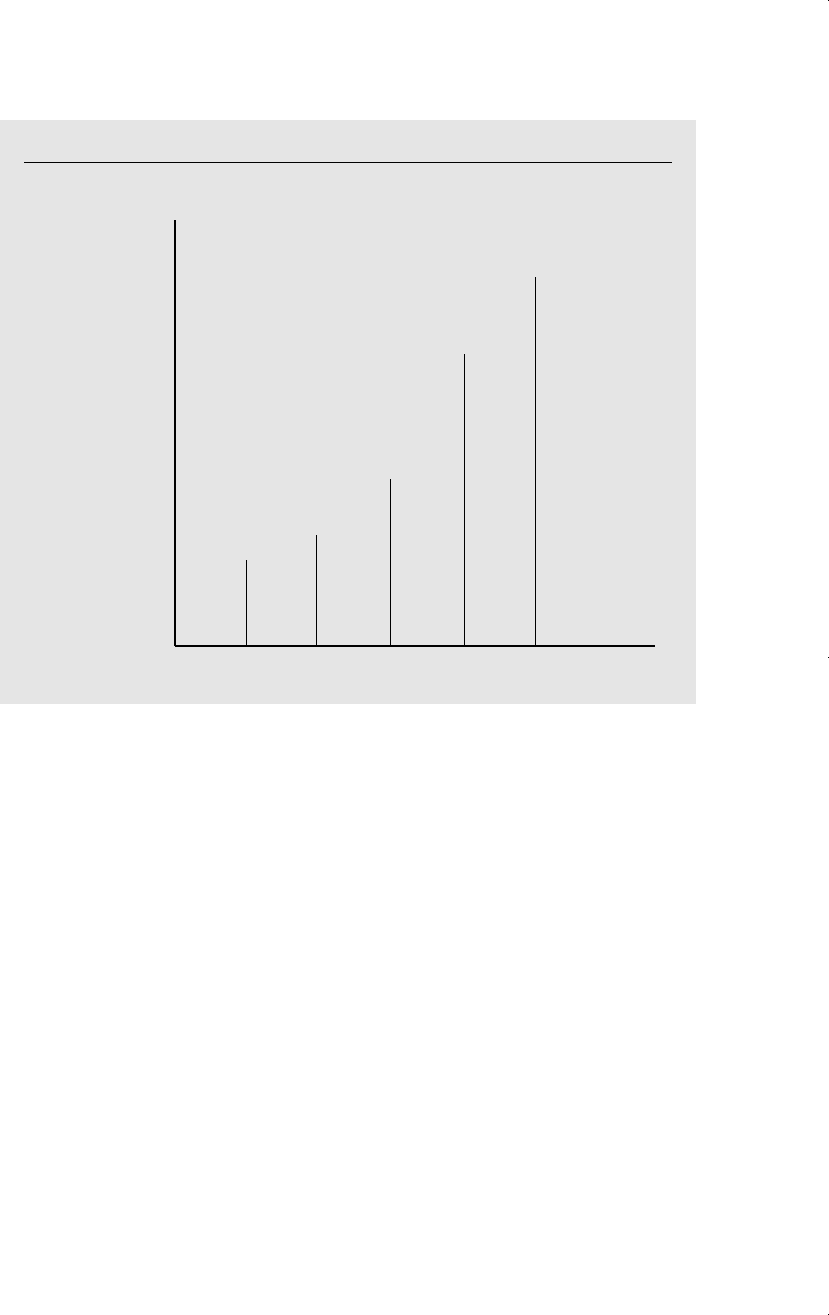
cation. Tracing out the expected value for various levels of education provides impor-
tant information on how wages and education are related. See Figure B.5 for an
illustration.
Appendix B Fundamentals of Probability
684
xd 7/14/99 8:57 PM Page 684

In principle, the expected value of hourly wage can be found at each level of edu-
cation, and these expectations can be summarized in a table. Since education can vary
widely—and can even be measured in fractions of a year—this is a cumbersome way
to show the relationship between average wage and amount of education. In economet-
rics, we typically specify simple functions that capture this relationship. As an exam-
ple, suppose that the expected value of WAGE given EDUC is the linear function
E(WAGE兩EDUC) 1.05 .45 EDUC.
If this relationship holds in the population of working people, the average wage for peo-
ple with eight years of education is 1.05 .45(8) 4.65, or $4.65. The average wage
for people with 16 years of education is 8.25, or $8.25. The coefficient on EDUC
implies that each year of education increases the expected hourly wage by .45, or 45
cents.
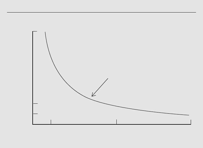
Conditional expectations can also be nonlinear functions. For example, suppose that
E(Y兩x) 10/x, where X is a random variable that is always greater than zero. This func-
tion is graphed in Figure B.6. This could represent a demand function, where Y is quan-
tity demanded, and X is price. If Y and X are related in this way, an analysis of linear
association, such as correlation analysis, would be inadequate.
Appendix B Fundamentals of Probability
685
Figure B.5
The expected value of hourly wage given various levels of education.
4 812
E(WAGE|EDUC)
16 20
EDUC
xd 7/14/99 8:57 PM Page 685

Properties of Conditional Expectation
Several basic properties of conditional expectations are useful for derivations in econo-
metric analysis.
PROPERTY CE.1:
E[c(X)兩X] c(X), for any function c(X).
This first property means that functions of X behave as constants when we compute
expectations conditional on X. For example, E(X
2
兩X) X
2
. Intuitively, this simply
means that if we know X, then we also know X
2
.
PROPERTY CE.2
For functions a(X) and b(X),
E[a(X)Y b(X)兩X] a(X)E(Y兩X) b(X).
For example, we can easily compute the conditional expectation of a function such as
XY 2X
2
:E(XY 2X
2
兩X) XE(Y兩X) 2X
2
.
The next property ties together the notions of independence and conditional expec-
tations.
PROPERTY CE.3
If X and Y are independent, then E(Y兩X) E(Y).
Appendix B Fundamentals of Probability
686
Figure B.6
Graph of E(Y
兩x) 10/x.
1 5 10
1
2
E(Y|x) 10
E(Y|x) = 10/x
x
xd 7/14/99 8:57 PM Page 686

This property means that, if X and Y are independent, then the expected value of Y given
X does not depend on X, in which case, E(Y兩X) always equals the (unconditional)
expected value of Y. In the wage and education example, if wages were independent of
education, then the average wages of high school and college graduates would be the
same. Since this is almost certainly false, we cannot assume that wage and education
are independent.
A special case of Property CE.3 is the following: if U and X are independent and
E(U) 0, then E(U兩X) 0.
There are also properties of the conditional expectation that have to do with the fact
that E(Y兩X) is a function of X,say E(Y兩X)
(X). Since X is a random variable,
(X)
is also a random variable. Furthermore,
(X) has a probability distribution and there-
fore an expected value. Generally, the expected value of
(X) could be very difficult to
compute directly. The law of iterated expectations says that the expected value of
(X) is simply equal to the expected value of Y. We write this as follows.
PROPERTY CE.4
E[E(Y兩X)] E(Y).
This property is a little hard to grasp at first. It means that, if we first obtain E(Y兩X) as
a function of X and take the expected value of this (with respect to the distribution of
X, of course), then we end up with E(Y). This is hardly obvious, but it can be derived
using the definition of expected values.
Suppose Y WAGE and X EDUC, where WAGE is measured in hours, and
EDUC is measured in years. Suppose the expected value of WAGE given EDUC is
E(WAGE兩EDUC) 4 .60 EDUC. Further, E(EDUC) 11.5. Then, the law of iter-
ated expectations implies that E(WAGE ) E(4 .60 EDUC) 4 .60 E(EDUC)
4 .60(11.5) 10.90, or $10.90 an hour.
The next property states a more general version of the law of iterated expectations.
PROPERTY CE.4ⴕ
E(Y兩X) E[E(Y兩X,Z)兩X].
In other words, we can find E(Y兩X) in two steps. First, find E(Y兩X,Z) for any other ran-
dom variable Z. Then, find the expected value of E(Y兩X,Z), conditional on X.
PROPERTY CE.5
If E(Y兩X) E(Y), then Cov(X,Y) 0 (and so Corr(X,Y ) 0). In fact, every function
of X is uncorrelated with Y.
This property means that, if knowledge of X does not change the expected value of Y,
then X and Y must be uncorrelated, which implies that if X and Y are correlated, then
E(Y兩X) must depend on X. The converse of Property CE.5 is not true: if X and Y are
uncorrelated, E(Y兩X) could still depend on X. For example, suppose Y X
2
. Then,
E(Y兩X) X
2
, which is clearly a function of X. However, as we mentioned in our dis-
cussion of covariance and correlation, it is possible that X and X
2
are uncorrelated. The
Appendix B Fundamentals of Probability
687
xd 7/14/99 8:57 PM Page 687

conditional expectation captures the nonlinear relationship between X and Y that corre-
lation analysis would miss entirely.
Properties CE.4 and CE.5 have two major implications: if U and X are random vari-
ables such that E(U兩X) 0, then E(U) 0, and U and X are uncorrelated.
PROPERTY CE.6
If E(Y
2
) and E[g(X)
2
] for some function g, then E{[Y
(X)]
2
兩X}
E{[Y g(X)]
2
兩X} and E{[Y
(X)]
2
} E{[Y g(X)]
2
}.
This last property is very useful in predicting or forecasting contexts. The first inequal-
ity says that, if we measure prediction inaccuracy as the expected squared prediction
error, conditional on X, then the conditional mean is better than any other function of X
for predicting Y. The conditional mean also minimizes the unconditional expected
squared prediction error.
Conditional Variance
Given random variables X and Y, the variance of Y, conditional on X x, is simply the
variance associated with the conditional distribution of Y, given X x: E{[Y
E(Y兩x)]
2
兩x}. The formula
Var(Y兩X x) E(Y
2
兩x) [E(Y兩x)]
2
is often useful for calculations. Only occasionally will we have to compute a condi-
tional variance. But we will have to make assumptions about and manipulate con-
ditional variances for certain topics in regression analysis.
As an example, let Y SAVING and X INCOME (both of these measured annu-
ally for the population of all families). Suppose that Var(SAVING兩INCOME) 400
.25 INCOME. This says that, as income increases, the variance in saving levels also
increases. It is important to see that the relationship between the variance of SAVING
and INCOME is totally separate from that between the expected value of SAVING and
INCOME.
We state one useful property about the conditional variance.
PROPERTY CV.1
If X and Y are independent, then Var(Y兩X) Var(Y).
This property is pretty clear, since the distribution of Y given X does not depend on X,
and Var(Y兩X) is just one feature of this distribution.
B.5 THE NORMAL AND RELATED DISTRIBUTIONS
The Normal Distribution
The normal distribution, and those derived from it, are the most widely used distribu-
tions in statistics and econometrics. Assuming that random variables defined over pop-
ulations are normally distributed simplifies probability calculations. In addition, we will
Appendix B Fundamentals of Probability
688
xd 7/14/99 8:57 PM Page 688

rely heavily on the normal and related distributions to conduct inference in statistics and
econometrics—even when the underlying population is not necessarily normal. We
must postpone the details, but be assured that these distributions will arise many times
throughout this text.
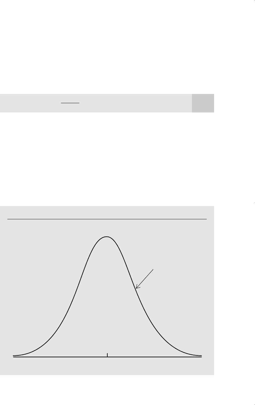
A normal random variable is a continuous random variable that can take on any
value. Its probability density function has the familiar bell shape graphed in Figure B.7.
Mathematically, the pdf of X can be written as
f(x) exp[(x
)
2
/2
2
], x , (B.34)
where
E(X), and
2
Var(X). We say that X has a normal distribution with
expected value
and variance
2
, written as X ~ Normal(
,
2
). Because the normal
distribution is symmetric about
,
is also the median of X. The normal distribution is
sometimes called the Gaussian distribution after the famous statistician C. F. Gauss.
Certain random variables appear to roughly follow a normal distribution. Human
heights and weights, test scores, and county unemployment rates have pdfs roughly the
shape in Figure B.7. Other distributions, such as income distributions, do not appear to
follow the normal probability function. In most countries, income is not symmetrically
distributed about any value; the distribution is skewed towards the upper tail. In some
1
兹
苶
2
Appendix B Fundamentals of Probability
689
Figure B.7
The general shape of the normal probability density function.
x
f
X
for a normal
random variable
xd 7/14/99 8:57 PM Page 689

cases, a variable can be transformed to achieve normality. A popular transformation is
the natural log, which makes sense for positive random variables. If X is a positive ran-
dom variable, such as income, and Y log(X) has a normal distribution, then we say
that X has a lognormal distribution. It turns out that the lognormal distribution fits
income distribution pretty well in many countries. Other variables, such as prices of
goods, appear to be well-described as lognormally distributed.
The Standard Normal Distribution
One special case of the normal distribution occurs when the mean is zero and the vari-
ance (and, therefore, the standard deviation) is unity. If a random variable Z has a
Normal(0,1) distribution, then we say it has a standard normal distribution. The pdf
of a standard normal random variable is denoted
(z); from (B.34), with
0 and
2
1, it is given by
(z) exp(z
2
/2), z . (B.35)
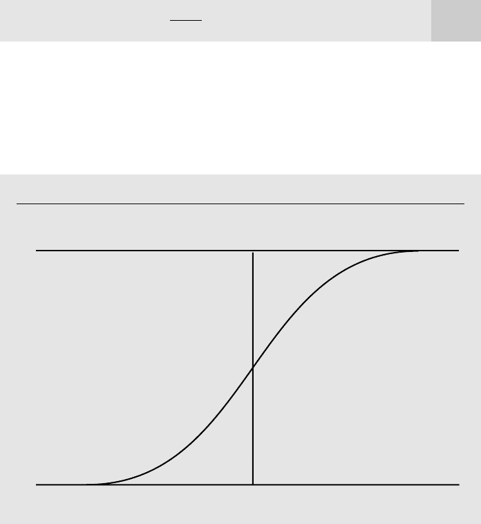
The standard normal cumulative distribution function is denoted (z) and is
obtained as the area under
, to the left of z; see Figure B.8. Recall that (z) P(Z
z); since Z is continuous, (z) P(Z z), as well.
There is no simple formula that can be used to obtain the values of (z) [because
(z) is the integral of the function in (B.35), and this intregral has no closed form].
1
兹
苶
2
Appendix B Fundamentals of Probability
690
Figure B.8
The standard normal cumulative distribution function.
0 z
1
0
.5
–3
3
xd 7/14/99 8:57 PM Page 690

Nevertheless, the values for (z) are easily tabulated; they are given for z between 3.1
and 3.1 in Table G.1. For z 3.1, (z) is less than .001, and for z 3.1, (z) is
greater than .999. Most statistics and econometrics software packages include simple
commands for computing values of the standard normal cdf, so we can often avoid
printed tables entirely and obtain the probabilities for any value of z.
Using basic facts from probability—and, in particular, properties (B.7) and (B.8)
concerning cdfs—we can use the standard normal cdf for computing the probability of
any event involving a standard normal random variable. The most important formulas
are
P(Z z) 1 (z), (B.36)
P(Z z) P(Z z), (B.37)
and
P(a Z b) (b) (a). (B.38)
Because Z is a continuous random variable, all three formulas hold whether or not the
inequalities are strict. Some examples include P(Z .44) 1 .67 .33,
P(Z .92) P(Z .92) 1 .821 .179, and P(1 Z .5) .692 .159
.533.
Another useful expression is that, for any c 0,
P(兩Z兩 c) P(Z c) P(Z c)
2P(Z c) 2[1 (c)].
(B.39)
Thus, the probability that the absolute value of Z is bigger than some positive constant
c is simply twice the probability P(Z c); this reflects the symmetry of the standard
normal distribution.
In most applications, we start with a normally distributed random variable, X ~
Normal(
,
2
), where
is different from zero, and
2
1. Any normal random vari-
able can be turned into a standard normal using the following property.
PROPERTY NORMAL.1
If X ~ Normal(
,
2
), then (X
)/
~ Normal(0,1).
Property Normal.1 shows how to turn any normal random variable into a standard nor-
mal. Thus, suppose X ~ Normal(3,4), and we would like to compute P(X 1). The steps
always involve the normalization of X to a standard normal:
P(X 1) P(X 3 1 3) P
冸
1
冹
P(Z 1) (1) .159.
X 3
2
Appendix B Fundamentals of Probability
691
xd 7/14/99 8:57 PM Page 691

EXAMPLE B.6
(Probabilities for a Normal Random Variable)
First, let us compute P(2 X 6) when X ~ Normal(4,9) (whether we use or is irrel-
evant because X is a continuous random variable). Now,
P(2 X 6) P
冸
冹
P(2/3 Z 2/3)
(.67) (.67) .749 .251 .498.
Now, let us compute P(兩X兩 2):
P(兩X兩 2) P(X 2) P(X 2) 2P(X 2)
2P
冸
冹
2P(Z .67)
2[1 (.67)] .772.
Additional Properties of the Normal Distribution
We end this subsection by collecting several other facts about normal distributions that
we will later use.
PROPERTY NORMAL.2
If X ~ Normal(
,
2
), then aX b ~ Normal(a
b,a
2
2
).
Thus, if X ~ Normal(1,9), then Y 2X 3 is distributed as normal with mean
2E(X) 3 5 and variance 2
2
9 36; sd(Y) 2sd(X) 23 6.
Earlier we discussed how, in general, zero correlation and independence are not the
same. In the case of normally distributed random variables, it turns out that zero corre-
lation suffices for independence.
PROPERTY NORMAL.3
If X and Y are jointly normally distributed, then they are independent if and only if
Cov(X,Y) 0.
PROPERTY NORMAL.4
Any linear combination of independent, identically distributed normal random vari-
ables has a normal distribution.
For example, let X
i
, i 1,2, and 3, be independent random variables distributed as
Normal(
,
2
). Define W X
1
2X
2
3X
3
. Then, W is normally distributed; we must
simply find its mean and variance. Now,
E(W ) E(X
1
) 2E(X
2
) 3E(X
3
)
2
3
0.
2 4
3
X 4
3
6 4
3
X 4
3
2 4
3
Appendix B Fundamentals of Probability
692
xd 7/14/99 8:57 PM Page 692
