Troyan V., Kiselev Y. Statistical Methods of Geophysical Data Processing

Подождите немного. Документ загружается.

Chapter 10

Construction and interpretation of

tomographic functionals

The recovery of the coeﬃcients, that are functions of space coordinates and describe

local properties of a medium from known characteristics of the sounding signal ﬁeld,

makes up the subject matter of inverse problems in the mathematical physics (Bel-

ishev, 1990; Blagoveshchenskii, 2005, 1978, 1966; Romanov, 1974, 1987; Faddeev,

1976; Newton, 1981). In setting up corresponding inverse problems, it is usual to

use the ﬁelds that are deterministically deﬁned on the space-time continuum as

initial data. A real experiment can be reduced to the traditional mathematical

setting, provided that the record is considered as continuous in time and the so-

called “reduction to an ideal device”, which is widely known the ill-posed problem

(Pytev, 1990; Tikhonov and Arsenin, 1977), is ﬁrst performed and then followed

by the space-time interpolation. Although such a procedure causes a loss of the

information, it is still applied in certain cases (Yanovskaya and Porokhova, 2004).

To formulate a mathematical model and to set up an inverse problem that is ade-

quate to a real physical experiment (to remote sensing, in particular), it is necessary

to take into account basic factors determining the model construction. The recovery

of ﬁelds of the required parameters of a medium from values of a set of functionals

of measurements is a natural mathematical model of interpreting physical experi-

ment. In interpretation problems, the conjugate space of linear functionals arises

that provided a mathematical model of linear devices recording the sounding signal.

As it will be shown in what follows, the conjugate space enables us to interpret the

structure of functionals that directly act on the ﬁelds of the parameters of interest

in clear physical terms. These functionals are called tomographic functionals.

10.1 Construction of the Model of Measurements

The ﬁrst step in solving of the inverse problem of remote sensing is the construction

of the model of the relationship between measurement data and unknown param-

eters of the medium. As a rule, the digital records provided by spatially located

receivers are used as initial data. The unknown parameters determining the prop-

erties of the medium are the elements (θ(x)) of functional spaces (Θ): θ(x) ∈ Θ; for

293

294 STATISTICAL METHODS OF GEOPHYSICAL DATA PROCESSING

instance, the ﬁelds of magnetic and gravitational anomalies, the ﬁelds of conduc-

tivity (σ(x)), the ﬁelds of elastic Lame parameters (λ(x) andµ(x)), of the density

(ρ(x)), etc. The measurement space is the space of functionals {h

} over the ﬁelds

of sounding signals (ϕ ∈ Φ); the model of measurements

: u

= H

(ϕ)

∆



|ϕ



where n = 1 ÷N is a number of digital samples of the receiving system and {h

} ∈

∗

A tomographic experiment is determined by a mapping Θ (R

) −→ R

of the

functional space into the measurement space. Here, experimental data include some

noise ε and functionals of the known parameter ﬁelds, i.e.,

= P

(θ) + ε

. (10.1)

Let the propagation process be described by a linear operator L

so that

ϕ = s, (10.2)

where

ϕ is the ﬁeld of the sounding signal; s is the source ﬁeld, and

: L

(αϕ + βψ) = αL

ϕ + βL

ψ.

The operator L

determines the properties of the medium θ. Mathematically, the

problem of interpretation of a tomographic experiment reduces to the recovery of

the operator L

from the measurement data. To ﬁnd the solution, it is necessary

to reconstruct the functionals P

∈ Θ

∗

, from the relations H

(ϕ(θ)) = P

(θ) and

the propagation law (10.2).

Assume that the ﬁeld ϕϕ is generated by a group of sources and it is recorded by

a receiver with a directional pattern Ω and a ﬁxed orientation of its principal lobe

e. Assuming the size of the receiver to be small as compared with the typical sizes

of the problem (the wavelength of the sounding signal and the characteristic scale of

the inhomogeneity), we consider the receiver as localized at a point. For example,

the complete set of experimental data in the seismic case will be obtained if we take

into account that the experiment involves J group of sources,3×K (K is the number

of receiver points) traces from each group, and L processed samples of digital records

of the seismogram. This yields N = 3 K J L samples. It should be noted that it is

not the ﬁeld ϕ

ϕ that is directly recorded, but the result of its transformation by the

apparatus function H of the recording channel, which involves time and amplitude

quantization. The most general model of the transformation of the sounding signal

by the recording channel is given by the linear convolution operator. We introduce

a through numbering of samples (n = 1 ÷N). Then individual sample of the digital

record can be represented in the form

= H

−1

s + ε

H : H

ϕ =

ZZZ

dxdτdΩh

, e; t

− τ, x

− x)ϕ(x, e, τ), (10.3)

Construction of tomographic functionals 295

e : e ∈ R

Here, all the unknown properties of the medium are included into the operator

−1

, and the experimental data are given by the result of the convolution of the

ﬁeld ϕϕ with the apparatus function h. The experimental value coincides with the

projection of the ﬁeld ϕ(x, t) onto the direction n only in the idealized problem

formulation (where h

−t) = δ(t −t

), which corresponds to an inﬁnite spectral

band of the receiver, never occurring in practice, and where the directional pattern

satisﬁes the condition h(e

, e) = h(e

, e)), and only if the random error ε is

absent. As a realistic model of the determinate part of a particular measurement

one may take the functional h

= h

(

ϕ), which can be considered as continuous, for

physical reasons, and as linear, for technical speciﬁcations. Due to nonlinearity of

the functional P

(θ) from (10.1) (even if an explicit expression for its action on the

ﬁeld θ is available and if ε

−→ 0), the solution is necessarily of the interpretational

form. As a rule, a linearization of the functional P

is the basic component of an

each iteration step. Let the medium be described by the ﬁeld Θ

= Θ

(x). Then

the measurement model (10.1) takes the form

= P

(Θ

) +

δθ



(δθ) + ˜ε

where ˜ε

includes both the random noise ε

, and the noise caused by the lineariza-

tion and related to the determinate part of the model.

For the ﬁeld Θ

the propagation equation L

ϕ = s is satisﬁed. We assume that

the unknown ﬁeld θ is close to the ﬁeld Θ

, i.e. θ = Θ

+ δθ, δθ  Θ

. Sometimes

the solution ϕ

can be obtained in the analytic form by using an approximate

method, for instance, by the ray method. The solution for the medium with the

parameter ﬁeld θ is given by the equality

ϕ =

+ L

−1

δL

ϕ (10.4)

(δL

= L

−L

is the perturbation operator). The equality (10.4) is a consequence

of the operator identity

−1

≡ L

−1

+ L

−1

− L

−1

for the representation ϕ = L

−1

We note that the above expression (10.4) can be obtained provided that the

ﬁeld ϕ

satisﬁes the homogeneous equation L

= 0. Writing the operator as

L = L

− δL

and the solution ϕϕ as ϕ = ϕϕ

+ δϕϕ, we obtain the equation

δϕ = δL

ϕ ,

i.e., the correction of the perturbed ﬁeld is described by the same equation as the

ﬁeld ϕ

in the reference medium, but now with the source s = δL

ϕ including,

along with the ﬁeld ϕ

, also the correction δϕ.

Taking into account (10.4), the general model (10.3) can be written in the form

= H



+ L

−1

δL



+ ε

. (10.5)

296 STATISTICAL METHODS OF GEOPHYSICAL DATA PROCESSING

Here the medium properties are reﬂected both in δL

and in the factor ϕ. Due to

dependence of ϕ upon δθ, the determinate part of the measurement model proves

to be nonlinear with respect to δθ. If δθ is small enough, i.e., if the condition

||H

−1

δL

(ϕϕ − ϕ

)||

E(ε

)

 1 (10.6)

is satisﬁed (E is the expectation operator), then in (10.5) ϕ can be replaced by ϕ

Physically, it is the validity of the inequality (10.6) that determines the adequacy of

the model u

(

ϕ) to the real measurement condition, i.e., the model error resulting

from replacing

ϕ by ϕ

in (10.5) is much smaller than the measurement error.

We analyze the norm of the linearization error by using the inequality

||HL

−1

δL

(ϕ − ϕ

)|| ≤ ||HL

−1

δL

||||ϕ −ϕ

||.

The norm of the diﬀerence between the ﬁelds ϕ and ϕ

is bounded by physical

considerations (since physical ﬁelds do not possess inﬁnite energy), i.e., ||ϕ −ϕ

|| ≤

c < ∞. The operator HL

−1

δL

is compact, since so is the operator H (the integral

convolution operator), that determines the space-time quantization. As δθ −→ 0,

we have ||HL

−1

δL

|| −→ 0, and condition (10.6) is trivially satisﬁed. Taking into

account (10.6), we rewrite model (10.5) in the modiﬁed form

= H

[ϕ

+ L

−1

δL

] + ˜ε

. (10.7)

The errors, including the linearization errors, are suppressed by the action of the

operator H

. Introducing the bilinear form



ξ|η



V,T,Ω

Ω

ξ(e, x, t) ∗ η(e, x, t) dx dΩ,

we rewrite (10.7) as follows:



|ϕ



V,T,Ω



−1

δL



V,T,Ω

+ ˜ε

(∗ is the time convolution sign, V is the sounded domain, T is the time interval of

measurements).

Reducing the experimental data by the known value

= P

(Θ

) ≡



|ϕ



V,T,Ω

then yields

˜u



−1

δL



V,T,Ω

+ ˜ε

, (10.8)

where ˜u

= u

− u

Construction of tomographic functionals 297

10.2 Tomographic Functional

From the perturbation operator δL

we single out the monotone function ν (δθ)

with respect to wish the perturbation operator is linear. Taking into account that

in many tomographic problems the operator δL

is near-local (for example, it is a

diﬀerential operator), we rewrite (10.8) in the form

˜u



−1

)

∗

|δL



V,T,Ω

+ ˜ε



∗



δν

δL





T,Ω

|ν(δθ)



+ ˜ε

, (10.9)

where G

= L

−1

;

δν

δL

δu

δν



∗



δν

δL





T,Ω

The integral kernel of the functional with respect to ν(δθ) will be called the

tomographic functional:



out

|ϕ



T,Ω

, (10.10)

where

= ϕ

is the incoming ﬁeld ϕ

: L

= s, in the known reference medium

;

out

: L

∗

out

= h

is the reverted outgoing ﬁeld “generated” by the receiver;

= (δ/δν)δL

is the operator of the interaction of the ﬁelds ϕ

and ϕ

out

Taking into account (10.10), we represent the model (10.9) in the form

˜u = P ν + ˜ε ,

˜u = ||˜u

, . . . , ˜u

, ˜ε = ||˜ε

, . . . , ˜ε

P =



| . . . hp

. . . . . .

| . . . hp

. . . . . .

| . . . hp



, ν =



|ν

. . .

|ν

. . .

|ν



The tomographic functional determines the inﬂuence of all elements of the spatial

region upon the n-th sampling of experimental data. It should be noted that in

traditional ray tomography the tomographic functional is singular and is localized

along the ray connecting the source and the receiver, and its weight to along this ray

is constant. In the diﬀraction tomography, however, even if the ray description is

applicable to the ﬁelds

and ϕ

out

, every element of the volume of the region under

investigation is linked to the receiver and the source by two ray trajectories. Here,

to every element of the spatial region its own weight, determined by the interaction

of the ﬁelds

, ϕ

out

) is attributed. It should be noted that mathematical methods

of the computer tomography are based on methods for solving problems of the

integral geometry, in which data (projections) are given by integrals of parametric

functions on manifolds of lower dimensions (rays, two-dimensional surfaces). By

contrast, in diﬀraction tomography, the supports of tomographic functionals belong

298 STATISTICAL METHODS OF GEOPHYSICAL DATA PROCESSING

to R

. We note that the main content of a tomographic experiment is relating to

the overlapping of supports of tomographic functionals, i.e., the information on one

and the same element of the volume is contained in the whole set of measurements.

The measurements are related to the changes in the localization of the group of

sources (ϕ

in (10.10)), to the location and orientation of the receiver, and to the

sampling (ϕϕ

out

in (10.10)) of the dynamic ﬁelds.

A priori data can be represented either in probabilistic or in determinate form,

for instance, the type of the spatial symmetry can be speciﬁed. The determinate

form of the representation of a priori information makes it possible to reduce the

tomographic functional to that in a space of lower dimension. Whenever the medium

is a priori assumed to be stratiﬁed homogeneous, the support of the tomographic

functional is one dimensional, whereas the corresponding tomographic functional is

the Radon projection of the generalized tomographic functional onto the vertical

direction. In the case of the spherical symmetry, the parameter of the kernel of the

tomographic functional is the radial coordinate.

10.3 Examples of Construction and Interpretation of Tomographic

Functionals

Now we consider some examples of the constructing and interpreting of tomographic

functionals.

10.3.1 Scalar wave equation

The operators L

and L

are of the following form:

= −∆ + c

−2

(x)

∂

∂t

= −∆ + c

−2

(x)

∂

∂t

= c

(x), θ = c(x), x ∈ R

, ν = ν(x) =



1 −



∂

∂t

, p =



out



∂

∂t





In this case the conjugate Green’s operator

∗

: G

∗

(x, x

; t −t

) = G(x

, x; −(t −t

))

determines wave propagation from the receiver in the reverse time. The support

of the tomographic functional in a homogeneous reference medium is concentrated

in a paraboloidal layer if the incoming wave is plane, and in an ellipsoidal layer

if the incoming wave is spherical (assuming a point-type receiver). The section

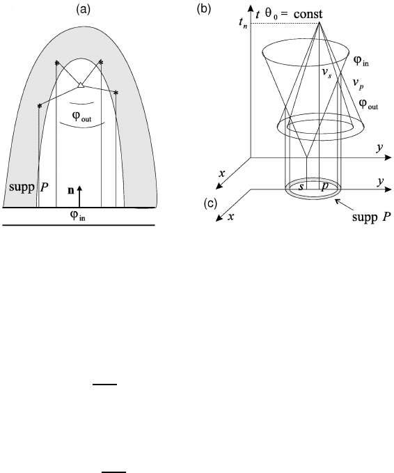
Construction of tomographic functionals 299

of the support of the tomographic functional passing through the symmetry axis

is shown in Fig. 10.1(a). Here the paraboloidal layer is formed by kinematically

equivalent points (c

=const). Fig. 10.1(b) sketches the conﬁguration of the support

of the tomographic functional under the assumptions that the source (s) is a point

one and the receiver (r) has the apparatus function h(t) = δ(t). The space-time

representations of the ﬁeld ϕ

and ϕ

out

, are shown in Fig. 10.1(b), and the support

of the tomographic functional is indicated in Fig. 10.1(c).

Fig. 10.1 Space-time representation of the ﬁelds and the support of the tomographic functional.

10.3.2 The Lame equation in an isotropic inﬁnite medium

The operators of the wave ﬁeld propagation in the reference (L

) and perturbed

) media are written as follows

ϕ = ρ

∂

∂t

− [(λ

+ µ

)∇

∇

∇ · ϕ + µ

∆ϕ + ∇∇λ

∇

∇ · ϕ

+ ∇µ

×∇∇ × ϕ + 2(∇∇µ

·∇∇)ϕ] ,

ϕ = ρ

∂

∂t

− [(λ + µ)

∇

∇ ·ϕ

ϕ + µ ∆ϕ

ϕ +

∇

∇λ

∇

∇ ·ϕ

+ ∇µ ×

∇

∇ × ϕ + 2(

∇

∇µ · ∇)ϕ] . (10.11)

Here

|λ

(x)



|µ

(x)



|ρ

(x)



, Θ =

|λ(x)



|µ(x)



|ρ(x)



ν(δθ) = δθ , λ(x) = λ

(x) + δλ(x) ,

300 STATISTICAL METHODS OF GEOPHYSICAL DATA PROCESSING

µ(x) = µ

(x) + δµ(x) ,

ρ(x) = ρ

(x) + δρ(x) .

In this case, the structure of the operator P can be described by the relation





= ||













||.

The perturbation operator δL = L

− L

from (10.4) is given by the sum

δL = δL

+ δL

where

δL

: δL

ϕ = δλ∇∇ ·ϕϕ +

∇

∇δλ∇ ·ϕϕ = ∇∇(δλ∇ · ϕ) , (10.12)

δL

: δL

ϕ = δµ

∇

∇ ·ϕ

ϕ + δµ∆ϕ

ϕ +

∇

∇δµ ×∇

∇

∇ ×

+ 2(

∇

∇δµ ·

∇

∇)ϕ

ϕ = 2δµ∆

ϕ + δµ ×

∇

∇ ×∇

∇

∇δµ ×∇

∇

∇ ×

ϕ + 2(∇

∇

∇δµ ·∇

∇

∇)ϕ

ϕ ,

δL

: δL

ϕϕ = −δρ

∂

∂t

ϕ . (10.13)

In the coordinate form with the unit vector e

, the expression (

∇

∇δµ · ∇)

ϕ can

be represented as the sum

(

∇

∇δµ ·

∇

∇ϕ

Using the identity

∇

∇ · (η

∇

∇ξ) = η∆ξ +

∇

∇η ·

∇

∇ξ ,

we transform the expression

2δµ∆

ϕ + 2(∇δµ · ∇)

to the form

∇

∇ · (δµ

∇

∇ϕ

In view of the identity

∇ × (ξf) = ∇ξ × f + ξ∇∇×f ,

we obtain

δµ∇ ×

∇

∇ × ϕ +

∇

∇δµ × ∇ × ϕ = ∇×δµ

∇

∇ × ϕ.

Finally, the action of the operator δL

is represented in the form

δL

∇

∇ × (δµ∇∇× ϕ) + 2∇∇· (δµ∇ϕ) .

Construction of tomographic functionals 301

We recall that the values of the tomographic functionals (10.10) allow for the

representation



|δθ



out

⊗ δL

dx.

For the variations of the arbitrary parameter ﬁeld δθ the symbol ⊗ denotes the

convolution over time and summation over all the indices of spatial coordinates

of vector and tensor expressions involved. The symbol ∗ is reserved for ordinary

convolution over time. For example,

⊗ ϕ

∆

= ψ

∗ δ

The determinate part ¯u

= ˜u

− ˜ε

of the model (10.9) can be represented as the

sum

¯u

out

⊗ δL

dx +

out

⊗ δL

ϕϕ

dx +

out

⊗ δL

ϕϕ

dx. (10.14)

Taking into account expression (10.12) for δL

, we single out the divergent part of

the ﬁrst integrand from (10.14)

out

⊗ δL

= ϕϕ

out

⊗ ∇(δλ∇ ·

)

≡ ∇∇· (ϕ

out

⊗ δλ

∇

∇ · ϕ

) − δλ∇ ·

out

⊗

∇

∇ϕϕ

and apply the Gauss–Ostrogradskii theorem, which yields

∇ · (ϕ

out

⊗ δλ∇ ·ϕϕ

)dx =

∂V

ds · (ϕϕ

out

⊗ δλ

∇

∇ · ϕ

Then we choose a large enough integration volume, which enables us to set δλ|

∂V

≡

0. Then the integral over the surface vanishes, and the ﬁrst term in (10.14) can be

rewritten as follows

out

⊗ δL

dx =

δλ∇

∇

∇ ·

out

⊗∇

∇

∇ ·

(x)δλ(x)dx = hhϕϕ

out

|ϕ

|δλi

: p



out

|ϕϕ



= −∇∇ · ϕ

out

⊗

∇

∇ · ϕ

, (10.15)

i.e., the action of the operator S

, describing the interaction of the ﬁelds ϕ

and

ϕϕ

out

, is reduced to the symmetric transformation of the ﬁelds ϕ

and ϕ

out

to the

ﬁelds of their divergences ∇∇ · ϕ

and ∇∇ · ϕ

out

. To determine the action of the

operator S

, we take into account the identity

∇ · (ξf) = ∇ξ · f + ξ∇ · f,

302 STATISTICAL METHODS OF GEOPHYSICAL DATA PROCESSING

and expression (10.13) for δL

. In this way we obtain the relation

out

⊗∇∇ · (δµ∇ϕ

)dx

∇

∇ · (ϕϕ

out

⊗ δµ

∇

∇ϕϕ

)dx −

∇ϕ

out

⊗ δµ∇ϕ

)dx . (10.16)

In view of the condition δµ|

∂V

= 0, the application of the Gauss–Ostrogradskii

theorem yields that the ﬁrst integral on the right hand side of the equation (10.16)

vanishes while the second integral involves δµ as a factor.

Similarly, the interaction of

out

with the second term in (10.16) yields

ϕϕ

out

⊗∇∇ × (δµ∇∇ × ϕ

) dx

∇ ·

out

(t − t

) × δµ∇ ×

)dx

(δµ∇ ×ϕϕ

out

⊗

∇

∇ × ϕ

)dx . (10.17)

Here, the ﬁrst integral on the right-hand side has the divergent form and vanishes

because δµ|

∂V

= 0. Finally, by using equations (10.16) and (10.17), we obtain

ϕϕ

out

⊗ δL

dx [∇ × ϕ

out

⊗ ∇ ×ϕϕ

− 2

∇

∇ϕ

out

⊗ ∇

]δµ

dxp

(x)δµ(x) = hhϕϕ

out

|ϕ

|δµi

i.e.,

: p



out

|ϕϕ



= ∇ ×

out

⊗ ∇ × ϕ

− 2∇

out

⊗∇∇ϕ

. (10.18)

In view (10.13), the action of the operator S

is determined by the expression

ϕϕ

out

⊗ δL

dx = −

out

⊗

∂

∂t

ϕϕ

dx , (10.19)

which can be rewritten in the form that is explicitly symmetric with respect to the

ﬁelds (

out

and

). Indeed, performing the integration by parts in (10.19)

ϕϕ

out

⊗

∂

∂t

∞

−∞

dtϕϕ

out

(T − t)

∂

∂t

ϕϕ

(t)

out

∂

∂t



∞

−∞

−

∂

∂t

out

∂

∂t