Steve M., Darby D.M., Geostatistics Explained - An Introductory Guide for Earth Scientists

Подождите немного. Документ загружается.

1,46

= 2.008, NS) and the regression line (Y = 295.26 – 1.56 X) is an extremely

poor ﬁt(Figure 21.6(a))withanr

of only 0.042. A plot of the unstandardized

residuals (Figure 21.6(b))conﬁrms the use of linear regression is inappropriate

because the data do not occur in a band around the horizontal line for zero

residual variation. Nor has the regression detrended the data; the plot of

residuals is similar to the original sequence with a pronounced long-term

non-linear trend. Finally, the correlogram of the residuals in Figure 21.6(c)

also shows highly signiﬁcant correlation at low and high lags, which conﬁrms

that there is remaining variation not explained by the regression.

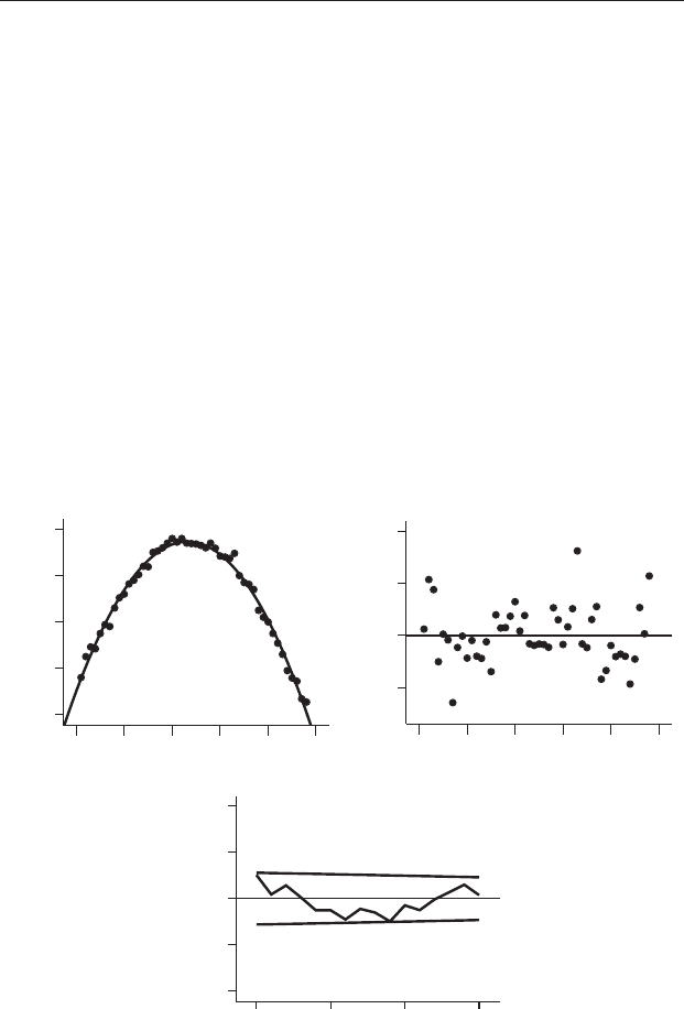
Second, a quadratic model (Equation (21.11): Y = 50.28 + 27.8 X – 0.60 X

)

ﬁtted to the data is highly signiﬁcant (F

2,45

= 2122.84, P < 0.001), and a far

better ﬁt than the linear model, with an r

of 0.989 (Figure 21.7(a)). A graph

of the residuals (Figure 21.7(b)) shows that the regression appears to be a

very good ﬁt to the data, and the correlogram of the residuals (Figure 21.7(c))

conﬁrms this, with no signiﬁcant autocorrelation at any lag.

Time

Turbidity

(a)

01020304050

400

300

200

100

Time

Residuals

(b)

01020304050

–20

(c)

number

11 16

1.0

0.5

0.0

–0.5

–1.0

Figure 21.7 Turbidity of water from well TGM013 in central Queensland

from early 2000 to late 2003. (a) A quadratic regression (heavy line) is a good ﬁt

to the points. (b) Unstandardized residuals. (c) Correlogram of the residuals for

a quadratic model ﬁtted to the data does not show signiﬁcant autocorrelation.

21.8 More complex regression 313

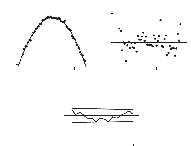
Finally, a cubic model (Equation (21.12): Y = 53.63 + 27.06 X – 0.56 X

–

0.001 X

)isalsosigniﬁcant (F

3,44

= 1392.67, P <0.001) with an r

of 0.990,

indicating a slight improvement over the quadratic and a very good ﬁttothe

data. The residuals and their correlogram are consistent with this (Figure 21.8).

In summary, both the quadratic and cubic polynomials are very good ﬁts

to the data and can account for almost all the change in the measured

variable over the sequence. There is a signiﬁcant non-linear relationship

between turbidity and time, with high turbidity during the middle part of

the sequence.

Even though the regression ﬁts the data, it cannot be used to predict

turbidity in the future because the values will be negative and negative

turbidity does not exist. We have deliberately chosen this example to

illustrate the danger of predicting beyond the measured limits of a

Time

Turbidity

(a)

01020304050

400

300

200

100

Time

Residuals

(b)

01020304050

–20

(c)

number

11 16

1.0

0.5

0.0

– 0.5

–1.0

Figure 21.8 Turbidity of water from well TGM013 in central Queensland

from early 2000 to late 2003. (a) A cubic regression (heavy line) is a good ﬁtto

the points, but appears little better than the quadratic in Figure 21.7.

(b) Unstandardized residuals. (c) The correlogram of the residuals does not

show signiﬁcant autocorrelation.

314 Introductory concepts of sequence analysis

sequence, but the same caution applies even when the predicted values

seem realistic.

From the value of r

, the linear model is a very poor ﬁttothedata.In

contrast, the quadratic is a good ﬁt and the cubic model is a slight improve-

ment over the quadratic. There is no point in using a more complex higher-

order polynomial if it does not give a signiﬁcantly improved ﬁt over a simpler

one, and this can be tested for signiﬁcance by a straightforward extension of

the ANOVA used to assess the signiﬁcance of a regression (Chapter 16). Most

statistical packages give a table of results for the ANOVA that tests for

departure from a line with zero slope (Chapter 16), which includes the sum

of squares, degrees of freedom and mean squares for the regression.

Table 21.1(a) gives these for the linear, quadratic and cubic models ﬁtted to

the data in Figures 21.6 to 21.8.

Each expansion of the polynomial is additive (e.g. Equations (21.10) to

(21.13)) and so are their sums of squares. Therefore, the sum of squares for

the improvement (if any) of the quadratic compared to the linear regression

can be obtained by subtracting the sum of squares for the linear model from the

sum of squares for the quadratic, giving the sum of squares for the diﬀerence

(SS diﬀerence). The number of degrees of freedom for the diﬀerence (df diﬀer-

ence) is also calculated by subtraction (Table 21.1(b)). The mean square for the

diﬀerence is (SS diﬀerence/df diﬀerence), and the F statistic is calculated by

dividing this quantity by the error of the higher polynomial (Table 21.1).

The same method is used to assess whether the cubic model is an

improvement compared to the quadratic. In the example in Table 21.1 the

additional variation explained by the quadratic over the linear model is

highly signiﬁcant, but the cubic model is not a signiﬁcant improvement over

the quadratic, so the latter is used to describe the relationship.

21.8.1 Polynomial modeling of a spatial sequence: hydrogen

diﬀusion in a single crystal of pyroxene

There are many common geological phenomena where polynomial approx-

imations are appropriate, particularly spatial data such as gravity models,

porosity, and other fundamental rock properties that vary with depth, shoreline

changes, as well as distortion and translation corrections in image analysis.

For example, diﬀerent types of diﬀusion processes are often described with

polynomials. Figure 21.9 shows data from an experiment to measure hydrogen

21.8 More complex regression 315

diﬀusion in a single crystal of pyroxene. A water-rich crystal was cooked in a

furnace so that hydrogen could diﬀuse out. After the experiment, the crystal

was sliced open, and the concentrationofhydrogenmeasuredfromedgeto

edge. The relationship between hydrogen concentration and location in the

crystal is best described by a third-order polynomial (Figure 21.9).

Table 21.1 The amount of additional variation explained by progressive polynomial

expansions can be assessed by subtracting the sum of squares for the lower

polynomial from the next higher one to give the sum of squares for the diﬀerence (SS

diﬀerence). The number of degrees of freedom for the diﬀerence (df diﬀerence) is also

obtained by subtraction. The mean square for the diﬀerence is (SS diﬀerence/df

diﬀerence), and the F statistic is calculated by dividing the resultant MS diﬀerence by

the error of the higher polynomial. (a) ANOVA statistics for each of the three

regression models. (b) ANOVA table for the relative importance of each additional

expansion of the regression equation. In this example the additional variation

explained by the quadratic model is a highly signi ﬁcant improvement over the linear

one, but there is no signiﬁcant improvement of the cubic model over the quadratic.

(a)

Model Sum of squares df Mean square

Linear (a) 5568.2 1 5568.2

Error 375 390.5 46 8160.7

Quadratic (b) 530 847.9 2 265 423.9

Error 5653.1 45 125.6

Cubic (c) 530 907.8 3 176 969.3

Error 5593.2 44 127.1

(b)

Model

Sum of squares

for the diﬀerence df

Mean square

of diﬀerence Error df F ratio

Quadratic

minus

(b) 530 847.9 2 Quadratic F

1,45

= 4182.2

linear (a) 5 568.2 1 P < 0.001

Diﬀerence 525 279.7 1 525 279.7 125.6 45

Cubic

minus

1,44

= 0.47

quadratic (b) 530 847.9 2 NS

Diﬀerence 59.9 1 59.9 127.1 44

316 Introductory concepts of sequence analysis

21.9 Simple autoregression

Often a correlogram will show signiﬁcant autocorrelation at low lags. This

may be because the series is non-stationary (e.g. Figure 21.3(d)), but for a

stationary series, or one that has been detrended, low lag autocorrelation

means there is a consistent relationship between successive values. For

example, a sequence might show a signiﬁcant dependence for the value of

the measured variable at time (t) on time (t − 1) (where t can be any point

within the sequence). This dependence can be modeled by autoregression

(meaning that the data set is regressed upon itself) and is of particular

interest in ﬁelds such as ﬁnance and meteorology, where sequence analysis

is used (with somewhat mixed success) in attempts to predict future

values.

Here is an example. In some parts of the world annual rainfall has been

found to be signiﬁcantly related to annual rainfall during the previous year,

or years (e.g. the value of the measured variable at time (t) is related to that

at (t − 1) or even (t − 2) or (t − 3)). Knowledge of this relationship, and its

reliability, might help predict future rainfall: Figure 21.10(a) shows annual

rainfall at the Neostrata 4 open cut coal mine in Western Australia from

1961–2008. During years when annual rainfall exceeds 350 mm the output

of the mine has to be reduced because of the accumulation of storm water

runoﬀ in the ﬂoor of the cut, so some indication of the rain expected

during the next year would help in planning extractive operations.

Figure 21.10(a) shows ﬂuctuation but no obvious longer-term trend, and

100

Distance (mm)

Hydrogen (ppm)

2345

Figure 21.9 Hydrogen concentration (in ppm) measured from edge to edge

across a single olivine crystal, after a dehydration experiment to characterize

the diﬀusivity of hydrogen. A cubic regression (heavy line) is a good ﬁt to the

points. The data and ﬁgure have been simpliﬁed from Woods et al.(2000).

21.9 Simple autoregression 317

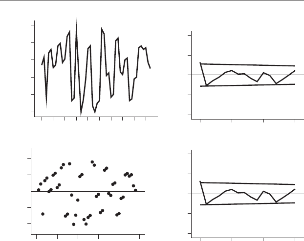
therefore a stationary series, which was conﬁrmed by the linear regression

having a slope close to zero (Y = 352.26 – 0.072 X : F

1,46

= 0.059, NS). The

regression is an extremely poor ﬁt(r

= 0.001). A correlogram of the

original data shows signiﬁcant positive autocorrelation at lag 1 and an

almost signiﬁcant negative autocorrelation at lag 2 (Figure 21.10(b)). A

scatter plot of the residuals against time is relatively evenly spread, but

nevertheless shows a pattern where the values for successive years are often

similar (Figure 21.10(c)). This was conﬁrmed by the correlogram of the

residuals, which is almost the same as the one for the original data

(Figure 21.10(d)).

First, considering the autocorrelation at lag 1, a regression equation

which only included autoregression on the previous year’s rainfall was ﬁtted

to the data:

400

380

360

340

320

300

1 6 11 16

(a)

21 26 31 36 41 46

Years since 1961

Rainfall

(b)

Lag number

11 16

1.0

0.5

0.0

–0.5

–1.0

(c)

Years since 1961

Residuals

01020304050

–25

–50

(d)

number

11 16

1.0

0.5

0.0

–0.5

–1.0

Figure 21.10 (a) Annual rainfall (in mm) for the Neostrata 4 mine, Western

Australia, from 1961–2008 inclusive. (b) Correlogram, of original data.

that (b) and (d) are extremely similar, thus showing that the linear regression

accounts for little variation in the data.

318 Introductory concepts of sequence analysis

¼ a þ B

t1

(21:14)

which was signiﬁcant (Y

= 237.08 + 0.323Y

t−1

: F

1,45

= 5.26, P < 0.05),

although the amount of variation explained by the regression was still low

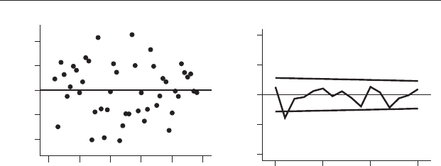
= 0.105). A graph of the residuals is more evenly distributed, but still

shows some similarity between successive values. A correlogram of the

residuals now shows no autocorrelation at lag 1, but signiﬁcant autocorre-

lation at lag 2 (Figure 21.11). The analysis was rerun, with the inclusion of a

second term to include the annual rainfall from two years before:

¼ a þ B

t1

þ B

t2

(21:15)

This too was signiﬁcant (Y

= 334.9 + 0.456Y

t−1

– 0.412Y

t−2

: F

2,43

= 7.43,

P < 0.01) and explains more than a quarter of the variation (r

= 0.257). Note

that for this example the constant for the ﬁrst lag is positive, but the one for

the second lag is negative, showing a positive relationship with the previous

year’s rainfall, but a negative one for the year before that.

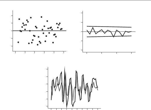
A graph of the residuals (Figure 21.12(a)) has a more even spread of

points and the correlogram of these residuals (Figure 21.12(b)) shows no

low lag autocorrelation (but two signiﬁcant values at higher lags). Finally,

although the rainfall predicted from Equation (21.15) is not identical to

actual rainfall, it is a surprisingly good predictor of years in the category

“rainfall exceeds 350 mm” and is therefore useful in planning extractive

operations at Neostrata 4 during the coming year (Figure 21.12(c)). This is

another example of how a complex sequence can be modeled by adding

additional terms to a regression equation.

(a)

Years since 1961

Residuals

01020304050

–25

–50

(b)

number

11 16

1.0

0.5

0.0

–0.5

–1.0

Figure 21.11 Autoregression analysis at t − 1 for the rainfall data at

Neostrata 4. (a) Residuals after autoregression at t − 1. (b) Correlogram of the

residuals. There is signiﬁcant negative autocorrelation remaining at lag 2.

21.9 Simple autoregression 319

21.10 More complex series with a cyclic component

Even a relatively complex time series can often be modeled, detrended and

interpreted using autocorrelation and regression. Figure 21.13 shows sea

level, measured in mm relative to a set reference point, at Port Magmago in

the Western Paciﬁc every December from 1960 to 2009. This relationship is

more complex than the previous examples. The sequence does not appear to

be stationary because sea level is generally lower during the middle, and

higher at the beginning and end of the sequence. There is also a marked

component of peaks and troughs.

A linear regression is clearly inappropriate for this non-stationary series,

so quadratic and cubic polynomials were ﬁtted in an attempt to model the

general trend. Both were signiﬁcant (Table 21.2) and explained about half

the variation despite the superimposed cyclic component.

(a)

Years since 1961

Residuals

01020304050

–25

–50

(b)

Lag number

11 16

1.0

0.5

0.0

–0.5

–1.0

400

380

360

340

320

300

3 8 13 18 23 28 33 38 43 48

(c)

Years since 1961

Rainfall

Figure 21.12 Autoregression analysis at t − 1 and t − 2 for the rainfall data at

Neostrata 4. (a) Residuals from an autoregression at t − 1 and t − 2.

(b) Correlogram of the residuals. The autoregression model has accounted for

the autocorrelation at low lags. (c) Actual rainfall (solid line), and predicted

rainfall (dashed line) from Equation (21.15).

320 Introductory concepts of sequence analysis

010

(a)

Year since 1960

Sea level (mm)

20 30 40 50

450

300

150

01020

(b)

Year since 1960

Residuals

40 50

150

100

–50

–100

(c)

number

11 16

1.0

0.5

0.0

–0.5

–1.0

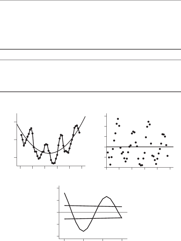
Figure 21.13 Data for sea level, in relation to a set reference point, at Port

Magmago from 1960 to 2009. There appears to be a cyclic component

superimposed over a trend that is not linear. (a) The quadratic line of best ﬁt

(heavy line) appears to approximate the overall trend, but not the strong cyclic

component. (b) Residuals are fairly evenly distributed about the line, showing

that the quadratic model has detrended the data, but there is still a cyclic

pattern with time. (c) A correlogram of residuals conﬁrms the strong cyclic

pattern remaining in the detrended data.

Table 21.2 Regression statistics for the linear, quadratic and cubic relationship ﬁtted

to the data for sea level shown in Figure 21.13. The value of r

is extremely low for the

linear relationship and the slope of the line is not signiﬁcant. In contrast, both the

quadratic and cubic relationships are signiﬁcant (P < 0.001 in each case) and both have

detected a signiﬁcant long-term change over time despite the cyclic component.

Equation r

F Probability ab

Linear 0.015 F

1,46

= 0.682 0.413 236.1 0.777 NA NA

Quadratic 0.499 F

2,45

= 22.453 < 0.001 382.8 −16.94 0.362 NA

Cubic 0.513 F

3,44

= 15.477 < 0.001 352.2 −9.59 −0.01 0.005

NA = not applicable because this term does not occur in the particular regression equation

21.10 More complex series with a cyclic component 321

The sums of squares for any improvement of the cubic over the quadratic,

and of the quadratic over the linear model, were calculated by subtraction

using the method in Table 21.1. This showed the cubic was not signiﬁcantly

better than the quadratic (F

1,44

= 1.26, NS), which was a highly signiﬁcant

improvement over the linear model (F

1,45

= 43.59, P < 0.001), so the quad-

ratic was used.

The quadratic line of best ﬁtinFigure 21.13(a) appears to follow the

general trend. The residuals are shown in Figure 21.13(b). A regression of

the residuals does not diﬀer signiﬁcantly from zero, which shows that the

quadratic has detrended the data to produce a stationary plot. Nevertheless,

the residuals still show a cyclic pattern and a correlogram of the residuals

still shows gross apparently cyclic autocorrelation (Figure 21.13(c)).

At this stage, you might decide the analysis is suﬃcient and conclude

that the sequence shows a signiﬁcant overall trend and a fairly regular

repetitive component. A more detailed regression model could include a

component based on a regular pattern such as a sine wave. These models are

described in more advanced texts and can be easily applied using statistical

software.

Finally, although the quadratic appears to be a good ﬁt to the overall trend

in the sequence, it may not be a reliable predictor of future sea level

(Figure 21.13(a)). Here too, we have deliberately used an example to

emphasize the risk of extrapolating outside the measured range of a variable.

21.11 Statistical packages and time series analysis

If you are working with a relatively simple time series, the methods given

here may be all you need. The availability of statistical software has made the

analysis of time series easy, especially when drawing correlograms and

applying complex regression models, but care is needed when interpreting

the results.

21.12 Some very important limitations and cautions

A correlogram gives the correlation coeﬃcient at numerous lags of the same

sequence. Therefore, even if the data in a sequence only vary at random, for

a signiﬁcance level of α you would expect this proportion of values of r to fall

outside the conﬁdence interval simply by chance. For example, with a

322 Introductory concepts of sequence analysis