Steve M., Darby D.M., Geostatistics Explained - An Introductory Guide for Earth Scientists

Подождите немного. Документ загружается.

describes the diﬀerences among samples. These new variables are called

principal components and are listed in decreasing order of importance

(beginning with the one that explains the most variation among sampling

units, followed by the next greatest, etc.). With a reduced number of variables,

any diﬀerences among sampling units are likely to be easier to visualize.

20.4 How does a PCA combine two or more variables

into one?

This is a straightforward example where data for two variables are combined

into one new variable, and we are using a simpliﬁed version of the conceptual

explanation presented by Davis (2002). Imagine you need to assess variation

within a large ore body for which you have data for the concentration of silver

and gold at ten sites. It would be helpful to know which sites were most

similar (and dissimilar) and how the concentrations of silver and gold varied

among them.

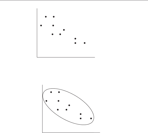
The data for the ten sites have been plotted in Figure 20.1 ,whichshows

a negative correlation between the concentrations of silver and gold. This

strong relationship between two variables can be used to construct a

single, combined variable to help make comparisons among the ten

sites. Note that you are not interested in whether the variables are

positively or negatively correlated – you onl y want to compare the sites.

The bivariate distribution of points for these two highly correlated

variables could be enclosed by a boundary. This is analogous to the way a

set of univariate data has a 95% conﬁdence interval (Chapter 8). For this

bivariate data set the boundary will be two dimensional, and because the

variables are correlated it will be elliptical as shown in Figure 20.2.

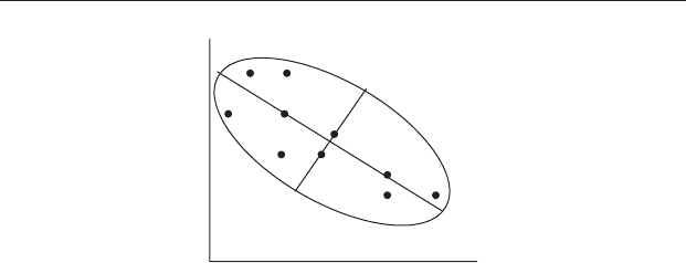
An ellipse is symmetrical and its relative length and width can be

described by the length of the longest line that can be drawn through it

Table 20.2 Because the concentrations of copper, silver, gold and zinc are

correlated, you only need data for one of these (e.g. silver), plus the concentration

of lead, to describe the diﬀerences among the sites.

Metal Site A Site B Site C Site D

Silver 11 40 28 19

Lead 46 63 26 21

20.4 Combining two or more variables 273

(which is called the major axis), and the length of a line drawn halfway down

and perpendicular to the major axis (which is called the minor axis)

(Figure 20.3).

The relative lengths of the two axes describing the ellipse will depend upon

the strength of the correlation between the two variables. Highly correlated

data like those in Figure 20.3 will be enclosed by a long and narrow ellipse, but

for weakly correlated data the ellipse will be far more circular.

At present the ten sites are described by two variables – the concentrations

of silver and gold. But because these two variables are highly correlated, all the

sites are quite close to the major axis of the ellipse, so most of the variation

among them can be described by just that axis (Figure 20.3). Therefore, you

can think of the major axis as a new single variable that is a good indication of

Gold

Silver

Figure 20.2 An ellipse drawn around the set of data for the concentration of

silver versus the concentration of gold in ore at ten sites. The elliptical

boundary can be thought of as analogous to the 95% conﬁdence interval for

this bivariate distribution.

Gold

Silver

Figure 20.1 The concentration of silver versus the concentration of gold at

ten sites.

274 Introductory concepts of multivariate analysis

most of the variation among sites. So instead of using two variables to

describe the ten sites, the information can be combined into just one.

The two axes are called eigenvectors and the relative length of each that

falls within the ellipse is its eigenvalue. Once the longest eigenvector of the

ellipse has been drawn, it is rotated (in the case of Figure 20.3 this will

simply be anticlockwise by about 45

) so that it becomes the new X axis

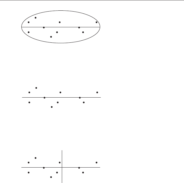
(Figure 20.4). This new, artiﬁcially constructed principal component

explains most of the variation among the ten sites. It has no name except

principal component number 1 (PC1). It is important to remember that

PC1 is a new variable – in this case it is a combination of the two variables

“concentration of silver” and “concentration of gold.” The plot of the points

in relation to PC1 in Figure 20.4 only shows the sites in terms of this new

variable – there is nothing about silver or gold in the graph.

The new X axis, PC1, is rescaled to assign the midpoint of the axis the

value of zero. This makes the axis symmetrical about zero, so the objects will

have both positive and negative coordinates for PC1 (Figure 20.5).

In this example, the points are all close to the major axis, so principal

component 1 explains the majority of the variation among the sites, and can

be used to easily assess similarities among them. From Figures 20.4 and 20.5

it is clear that sites A, I and F are more similar to each other than A is to E

because the distance between the former three is much shorter.

Because there are two variables in the initial data set, principal components

analysis also constructs a second component that is completely independent

and uncorrelated with principal component 1. The second axis is called

principal component 2 (PC2) and is simply the minor axis of the ellipse

Gold

Silver

Figure 20.3 The long major axis and shorter minor axis give the dimensions

of the ellipse that encloses the set of data.

20.4 Combining two or more variables 275

shown in Figure 20.3, which after the rotation described above will be a line

perpendicular to PC1. Here too, the eigenvalue for PC2 corresponds to its

relative length and its midpoint is given the value of zero. It is clear that PC2

does not explain very much of the variation among the sites – the objects are

quite widely dispersed around it, so it is a relatively short eigenvector

(Figure 20.6). Therefore, most of the variation is described by PC1, and the

analysis has eﬀectively reduced the number of variables from two to one.

20.5 What happens if the variables are not highly correlated?

As described above, if the two variables are highly correlated the ellipse

enclosing the data will be very long and narrow. Therefore the ﬁrst

PCI

–1.5 –1.0 1.0 1.50

Figure 20.5 The values for PC1 are expressed in relation to the midpoint of

the principal eigenvector, which is assigned the value of zero.

PCI

I H

Figure 20.4 The long axis of the ellipse has been drawn through the set of

highly correlated data for the concentration of silver and the concentration of

gold (Figure 20.3), and then rotated to give a new X axis (which is the major

axis of the ellipse) for the arti ﬁcial variable called principal component

number 1. This new variable explains most of the variation among sites.

PC2

PC1

Figure 20.6 Principal component 2 is the short axis of the ellipse shown in

Figure 20.5 and constructed by drawing a line perpendicular to the line

showing PC1. Note that PC2 explains very little of the variation among sites.

276 Introductory concepts of multivariate analysis

eigenvector will be relatively long with a large eigenvalue, and the second

will be relatively short with a small eigenvalue. In this case, by itself the new

combined variable of the ﬁrst eigenvector is a good indicator of the

diﬀerences among sites.

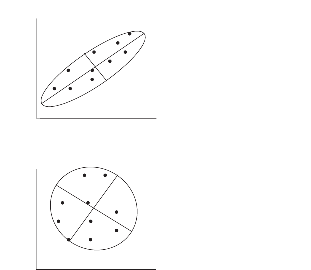
In contrast, if the two variables are not correlated the ellipse will be more

circular and the ﬁrst and second eigenvectors will both have similar eigen-

values (Figure 20.7). Therefore, neither can be used by themselves as a

good indication of the diﬀerences among sites.

20.6 PCA for more than two variables

Principal components analysis becomes particularly useful when you have

data for three or more variables.

(a)

(b)

Figure 20.7 (a) Highly correlated data. The long axis is a good indication of

variation among sites. (b) Uncorrelated data. The major and minor axes of the

ellipse surrounding the data points are both similar in length. Therefore

neither axis is a good single summary of the variation among sites.

20.6 PCA for more than two variables 277

If you have n variables a PCA will calculate n eigenvectors (with

n eigenvalues) that give the dimensions of an n-dimensional object in an

n-dimensional space. This may sound daunting but it is easy to visualize for

only three variables, where the three eigenvectors will give the dimensions

for a three-dimensional object in three-dimensional space. The object will

be close to spherical for a data set with no correlations and therefore little

redundancy, but a very elongated three-dimensional hyperellipsoid for a set

of two or three highly correlated variables. The same applies to however

many additional dimensions there are.

For three or more variables the PCA procedure is an extension of the

explanation given for two variables in Section 20.4.

The longest axis of the object is found and rotated so that it becomes the

X axis lying horizontally to the viewer on a two-dimensional plane with its

ﬂat surface facing the viewer (like the page you are reading at the moment).

If there are many variables and therefore many dimensions, the rotation is

likely to be complex – for example, an eigenvector in three dimensions may

have to be rotated in both the transverse and the horizontal. The eigenvector

for the longest axis then becomes principal component 1.

After this the other eigenvectors are drawn. For example, if you have

measured three variables, then the three-dimensional boundary enclosing

the data points will have three eigenvectors describing its length, breadth

and depth, all at 90° to each other.

In many cases several variables may be highly correlated with each other,

so the hyperellipsoid may be relatively simple and may even describe most

of the variation among sites in just one or two dimensions.

Here is an example. An environmental geochemist sampled sediments

along a 100 mile section of coastline, including ﬁve estuaries (A–E) that

received storm water runoﬀ from urban areas and ﬁve control estuaries

(F–J) that did not. At each site, they obtained data for the concentration of

copper, lead, chromium, nickel, cadmium, aluminum, mercury, zinc, total

polycyclic aromatic hydrocarbons (ΣPAHs) and total polychlorinated

biphenyls (ΣPCBs). These ten variables were subject to principal compo-

nents analysis and re-expressed as ten principal components giving the

shape of a ten-dimensional hyperellipsoid. Because several of the initial

variables were highly correlated, the ﬁrst principal component (PC1)

explained 70% of the variation among estuaries. The second, PC2,

explained 15% more of the variation and the third, PC3, only 5% of the

278 Introductory concepts of multivariate analysis

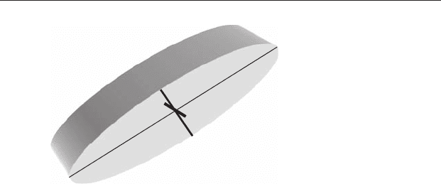
variation. Therefore, in this case 85% of the variation among site could be

described by a two-dimensional ellipse with axes of PC1 and PC2, and 90%

could be described by a three-dimensional ellipse with axes of PC1, PC2 and

PC3. So the three-dimensional hyperellipsoid will approximate a very

elongate, not very wide, and even less thick object suspended in three-

dimensional space (Figure 20.8) and the remaining seven dimensions will

make little contribution to its shape.

Therefore, you could take only PC1 and PC2 and plot a two-dimensional

ellipse from which you can easily visualize the relationships among the sites.

The two principal components explain 85% of the variation, so the closeness

of the objects in two dimensions will give a realistic indication of their

similarities (Figure 20.9). The analysis shows two relatively distinct clusters

corresponding to the ﬁve urban and ﬁve control estuaries, consistent with

urban storm water runoﬀ having a relatively consistent eﬀect (although you

need to bear in mind that this is only a mensurative experiment).

20.7 The contribution of each variable to the principal

components

Although the analysis described above has reduced the ten variables to two

principal components, it is often useful to know which speciﬁc variables

contribute to each of these components. For example, most of the variation

(i.e. PC1) might only be related to ΣPAHs and ΣPCBs; such an outcome

might suggest ways of reducing the eﬀects of urban development upon

PC2

PC1

PC3

Figure 20.8 Because several variables are highly correlated they can be re-

expressed as a hyperellipsoid with one very long axis (PC1), a shorter one

(PC2) and a very short one (PC3). Most of the variation can be explained by

PC1 and PC2. The third component, PC3, accounts for very little variation

and could be ignored.

20.7 The contribution of each variable 279

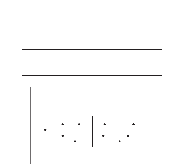
estuaries. To address questions such as these, PCA also gives the relative

contribution of each variable to each component.

The output from a PCA usually includes a plot such as Figure 20.9 and a

table of eigenvalues. As described above, an eigenvalue gives the relative

length of each eigenvector for the dimensions of the hyperellipsoid. As an

example, a list of eigenvalues is given in Table 20.3, which also gives the

percentage of variation explained by each principal component. Here too

the hyperellipsoid is non-spherical, so you know the variables show redun-

dancy and the PCA procedure has usefully reduced the number of variables.

Importantly, as well as reducing the number of variables to help visualize

the relationships among objects, PCA also gives the relative contribution of

the original variables to each eigenvalue. The output table from a PCA will

contain a list of the original variables and their correlations with each of the

principal components. Table 20.4 gives an example for the ten variables in the

Table 20.3 Typical output table for only the ﬁrst three

components of a PCA. PC1 explains most (70%) of the

variation in the data set and thus has the largest eigenvalue.

Principal component Eigenvalue Percentage variation

1 3.54 70

2 1.32 15

3 0.64 5

–1

–2 –1 0 1 2

PC2

PC1

Figure 20.9 A plot of only PC1 and PC2 can still explain most of the

variation among sites A–J. Note that the ﬁve urban estuaries are clustered to

the right of the plot and the ﬁve control estuaries are clustered to the left.

280 Introductory concepts of multivariate analysis

estuarine study described above. It is clear that principal component 1 is

mainly composed of variables 3 and 6, which are chromium and aluminum

(the two highest positive and negative correlations). In contrast, principal

component 2 is largely composed of variables 1, 2 and 10, which are copper,

lead and ΣPCBs. Which two variables make the major contribution to

principal component 3? You need to look for the highest correlations,

irrespective of their signs. (They are nickel and cadmium.)

The signs of the correlations are also useful. For example, for principal

component 1 (Table 20.4), the correlation coe ﬃcient for variable 3 (chro-

mium) is positive, and the one for variable 6 (aluminum) is negative. This

means that as PC1 increases, chromium concentration also increases, but

aluminum decreases.

In summary, a PCA has the potential to express multivariate data in a

form that we can more easily understand, by reducing the number of

dimensions so the data can be plotted on a two- or three-dimensional

graph. It also gives a good indication of which variables contribute most

to the diﬀerences among sampling units.

Table 20.4 Typical output table from a PCA. The far left-hand column lists the

original variables (in this case, variables 1–10) and the elements they represent. The

next three columns represent the ﬁrst three principal components and the values in

these columns are the correlations between the new components and the original

variables. Note that PC1 is primarily composed of the concentrations of variables 3

and 6 (the two largest values for the correlation coeﬃcients and shown in bold) while

PC2 is primarily composed of the concentrations of variables 1, 2 and 10 (also bold).

The variables that contribute most to PC3 are 4 and 5.

Original variable Component 1 Component 2 Component 3

1 Copper 0.01 0.60 0.22

2 Lead 0.24 0.61 0.37

3 Chromium 0.91 0.26 −0.06

4 Nickel −0.18 0.32 0.57

5 Cadmium 0.15 0.05 0.52

6 Aluminum −0.87 −0.22 0.44

7 Mercury 0.42 0.19 0.37

8 Zinc 0.30 −0.02 −0.22

9 ΣPAHs −0.17 0.21 −0.06

10 ΣPCBs 0.05 −0.71 0.32

20.7 The contribution of each variable 281

20.8 An example of the practical use of principal

components analysis

A marine geochemist was interested in comparing the hydrocarbons

in sediments at six sampling sites, each one mile apart, running south

along the shore and increasingly distant from a petrochemical plant to

(a) see if there were diﬀerences in hydrocarbon levels among the sites, and

(b) if so, to ﬁnd out which compounds might be the best indicators of

pollution.

The geochemist sampled ten hydrocarbons at each of six sites (A–F). A

principal components analysis showed that only two hydrocarbons, 1 and 6

(combined as PC1), contributed to most of the variation among sites and

were negatively correlated with PC1, followed by 5 and 9 (combined as

PC2). When plotted on a graph of PC1 and PC2 there was a clear pattern

(Figure 20.10) in that the rank order of the sites, running from left to right,

corresponded to their distance from the petrochemical plant. Thus they

concluded that the concentrations of only two hydrocarbons can explain

most of the variation among sites.

20.9 How many principal components should you plot?

There are several ways of deciding upon how many components to use in a

plot. If you are lucky, you might be in the situation where only one or two

are needed, but this will only occur if they account for almost all the

percentage variation among sampling units. Generally, however, you

should not use components with eigenvalues of 1.0 or less, because this

is the level of variation that you would expect by chance when there are no

strong correlations among variables and therefore all original variables

contribute equally to a component.

PC2

(A)

(B)

(C)

(D)

(E)

(F)

PC1

Figure 20.10 A plot of PC1 and PC2 for six sites increasingly distant (site

A = closest, site F = most distant) from a petrochemical plant. The analysis

shows a clear gradation through sites A to F.

282 Introductory concepts of multivariate analysis