Stefanica D. Solutions Manual: A Primer For The Mathematics Of Financial Engineering
Подождите немного. Документ загружается.


54
CHAPTER
2.
NUMERICAL
INTEGRATION.
BONDS.
2.1.
SOLUTIONS
TO
CHAPTER
2
EXERCISES
55
The
data
below refers
to
the
pseudocode from Table 2.7 of
[2]
for computing
the
price,
duration
and
convexity of a
bond
given
the
yield of
the
bond.
Input:
n =
5;
y = 0.07;
I 2 5 8
11
141
t_c
础且
ow
=
11-2
1~2
1~2
~;
~;
I;
v_cash_flow =
[2
2 2
2
叫
ac
∞
ou
叩
po
∞
np
归
ay
尼
rrr
江即
I
payment.
口
Output:
bond
price B =
10
1.
704888,
bond
duration
D =
1.
118911,
and
bond
convexity C =
1.
285705.
口
Problem
14:
By how much would
the
price of a
ten
year zero-coupon
bond
change if
the
yield increases by
ten
basis points? (One
perce
时
age
poi
时
IS
equal
to
100 basis points.
Thus
, 10 basis points is equal
to
0.00
1.)
Solution:
The
duration
of a
zero-coupo
丑
bond
is equal
to
the
maturity
of
the
bond
, i.e., D = T = 10. For small changes
!:1
y in
the
yield,
the
percentage
change in
the
value of a
bond
can
be
estimated as follows:
!:1
B
王一目
-!:1
y
D = … 0.001 . 10 = - 0.0
1.
We conclude
that
the
price of
the
bond
decreases by
1%.
口
Problem
12: Compute
the
price,
duration
and
convexity of a two year
semiannual coupon
bond
with
face value 100
and
coupon
rate
8%
,if
the
zero
rate
curve is given by
r(O
,t) = 0.05 + O.Olln
(1
+
~)
Solution:
The
data
below refers
to
the
pseudocode from Table 2.5 of
[2]
for
computing
the
price of a
bond
given
the
zero
rate
curve.
Input:η=
4;
zero
rateγ
(0
,
t) = 0.05 + O.Olln
(1
十
i);
t_cash
一丑
ow
=
[0.5
1
1.
5
2]
;
v_cash
且
ow
=
[4
4 4
104]
.
disc = [0.97422235 0.94738033 0.91998838 0.89238025].
Output:
Bond price B = 104.17391
1.
Note: To compute
the
duration
and
convexity of
the
bond
,
the
yield would
have
to
be
known.
The
yield
can
be
computed
, e.g., by using Newton's
method
, which is discussed
in
Chapter
8.
We
obtain
that
the
yield of
the
bond
is 0.056792, i.e., 5.6792%,
and
the
duration
and
convexity of
the
bond
are D =
1.
8901
and
C = 3.6895,
respectively.
口
Problem
15:
A five year
bond
with
duration
3~
years is worth 102.
Find
an
approximate price of
the
bond
if
the
yield decreases by fifty basis points.
Solution: Note
that
, since
the
yield of
the
bond decreases,
the
value of
the
bond
must
increase.
Recall
that
the
percentage change in
the
price of
the
bond
can
be
approx-
imated
by
the
duration
of
the
bond
multiplied by
the
parallel shift in
the
yield curve,
with
opposite sign, i.e.,
!:1
B
万一句
-
!:1
y D
For B = 102, D = 3.5
and
!:1
y =
-0.005
(since
1%
= 100 bp),
we 五
nd
that
!:1
B
用
-
!:1
y D B =
1.
785.
The
new value
of
the
bond
is
Discount factors:
Problem
13:
If
the
coupon
rate
of a
bond
goes up,
what
can
be
said
about
the
value of
the
bond
and
its duration? Give a financial argument. Check
your answer mathematically
,i.e.,by
cor
叩灿
gggand
gg7and
ShhO
叭仰飞
w
咄
ν
these
f
旬
Ul
丑
nc
囚
ctior
丑
IS
are either always positive or always
1
丑
lega
肮,
ti
忖
ve.
Solution:
If
the
coupon
rate
goes
up
,
the
coupon payments increase
and
therefore
the
value of
the
bond
increases.
The
duration
of
the
bond
is
the
time
weighted average of
the
cash flows,
discounted
with
respect
to
the
yield of
the
bond.
If
the
coupo
日
rate
increases,
the
duration
of
the
bond
decreases.
This
is due
to
the
fact
that
the
earlier
cash flows equal
to
the
coupo
丑
payments
become a higher fraction of
the
payment made
at
maturity
,which is equal
to
the
face value of
the
bond
plus
B
new
-
B +!:1B -
103.75.
口
Problem
16:
Establish
the
following relationship between
duration
and
convexity:
叮
θD
C _ D
:t.
-
-=:.一
oy
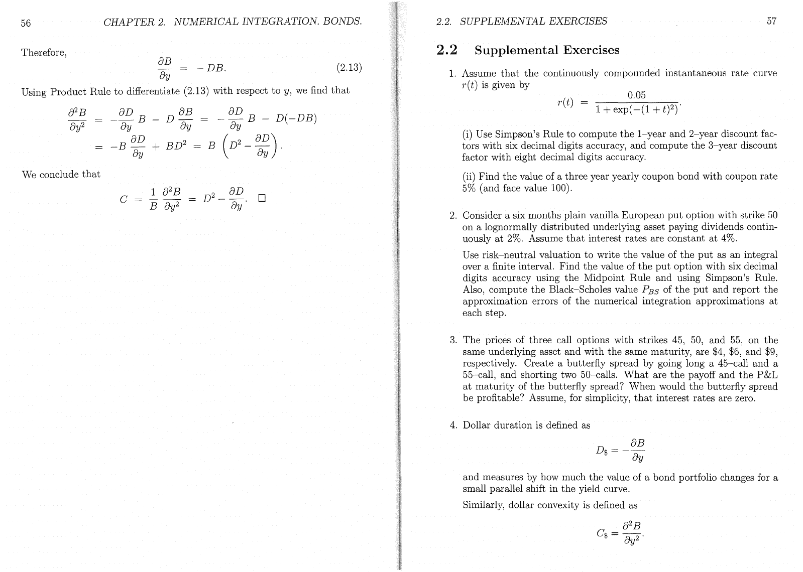
Solution: Recall
that
C
,d
a
B-vu
l-DU
D
1θ
2B
B
θ
y2
56
CHAPTER
2.
NUMERICAL
INTEGRATION.
BONDS.
2.2.
SUPPLEMENTAL
EXERCISES
57
Therefore,
θB
一一
=
-DB.
θν
Using
Product
Rl
由
to
differentiate (2.13)
with
respect
to
y,
we
直
nd
that
2.2
Supplemental
Exercises
(2.13)
1.
Assume
that
the
continuously compounded instantaneous
rate
curve
γ
(t)
is given by
γ
(t)
= 0.05
exp(
一
(1
+
t)2)
.
B
D
D
-D-hu
no-rC
DB
B-2
:-uu
C
1θ
2B
B
θν2
D2_
~D.
0
θu
(i) Use
Simpsor
内
Rule
to
compute
the
1-year
and
2-year discount fac-
tors
with
six decimal digits accuracy,
and
compute
the
3-year discount
factor
with
eight decimal digits accuracy.
(ii)
Find
the
value of a three year yearly coupon bond with coupon
rate
5%
(and face value 100).
We conclude
that
2.
Consider a six months plain vanilla European
put
option with strike
50
on a lognormally distributed underlying asset paying dividends contin-
uously
at
2%.
Assume
that
interest rates are constant
at
4%.
Use
risk-neutral
valuation
to
write
the
value of
the
put
as
an
integral
over a finite interva
l.
Find
the
value of
the
put
option with six decimal
digits accuracy using
the
N
Ii
dpoint Rule
and
using Simpson's Rule.
Also
, compute
the
丑
lack-Scholes
value
PBS
of
the
put
and report
the
approximation errors of
the
numerical integration approximations
at
each step.
3.
The
prices of three call options with strikes
45
,
50
, and
55
, on
the
same underlying asset
and
with
the
same
maturity
, are
$4
,
$6
, and
$9
,
respectively. Create a butterfly spread by going long a 45-call
and
a
55-call
,
and
shorting two 50-calls.
What
are
the
payoff and
the
P
&L
at
maturity
of
the
butterfly spread?
When
would
the
butterfly spread
be profitable? Assume
,for simplicity,
that
interest rates are zero.
4.
Dollar
duration
is defined as
D
电=一旦
ωθu
and measures by how much
the
value of a bond portfolio changes for a
small parallel shift in
the
yield curve.
Similarly
, dollar convexity is defined as
C
虫二工
θ
2B
eθy2·

58
CHAPTER
2.
NUMERICAL
INTEGRATION.
BONDS.
2.3.
SOLUTIONS
TO
SUPPLEJYIENTAL
EXERCISES
59
Note
that
, unlike classical
duration
and
convexity, which can only
be
computed for individual bonds,dollar duration
and
dollar convexity can
be
estimated for any bond portfolio, assuming all bond yields change
by
the
same amount. In particular, for a bond
with
value B,
duration
D ,
and
convexity C,
the
dollar
duration
and
the
dollar convexity can
be
computed as
D$
=
BD
and
G$
=
BG.
You invest
$1
million in a
bond
with
duration 3.2
and
convexity
16
and
$2.5 million
in
a bond with
duration
4
and
convexity
24.
(i)
What
are
the
dollar
d
旧
ation
and
dollar convexity of your portfolio?
(ii)
If
the
yield goes up
by
ten
basis
points
,五叫
new
approximate values
for each of
the
bonds.
What
is
the
new value of
the
portfolio?
(iii) You can buy or sell two
other
bo
时
s
,
one
with
d
旧时
ion
1.
6
and
convexity
12
and
another one
with
duration
3.2
and
convexity
20.
What
positions could you take in these bonds
to
immunize your portfolio
(i.
e.
,
to
obtain
a portfolio
with
zero dollar
duration
and
dollar
co
盯
exity)?
2.3
Solutions
to
Supplemental
Exercises
Problem
1: Assume
that
the
continuously compounded instantaneous
rate
curve r(t) is given by
γ
(t)
二
0.05
xp(
一
(1
+
t)2)
.
Use Simpson's Rule
to
compute
the
1-year
and
2-year discount factors
with
six decimal digits accuracy,
and
compute
the
3-year discount factor
with
eight decimal digits accuracy.
(ii)
Find
the
value of a three year yearly coupon
bond
with
coupon
rate
5%
(and face value 100).
Solution: (i) Recall
that
the
discount factor corresponding
to
time
t is
叫-fa'州市
Using Simpson's Rule,
we
obtain
that
the
1-year
, 2-year,
and
3-year
discount
factors are
disc(l)
= 0.956595; disc(2) = 0.910128; disc(3) = 0.86574100.
(ii)
The
value of
the
three year yearly coupon
bond
is
B = 5 disc(l) +5 disc(2) +105 disc(3) =
100.236424.
口
Problem
2: Consider a six months
plai
丑
vanilla
European
put
option with
strike
50
on a lognormally distributed underlying asset paying dividends
co
坠
tinuouslyat
2%.
Assume
that
interest rates are constant
at
4%.
Use
risk-neutral
valuation
to
write
the
value of
the
put
as
an
integral
over
a
且
nite
interval.
Find
the
value of
the
put
option
with
six decimal digits
accuracy using
the
Midpoint Rule
and
using Simpson's Rule. Also,compute
the
Black-Scholes value PBS of
the
put
and
report
the
approximation errors
of
the
numerical integration approximations
at
each step.
Solution:
If
the
underlying asset follows a lognormal distribution,
the
value
S(T)
of
the
underlying asset
at
maturity
is a lognormal variable given by
/σ2\
广-
In(S(T))
=
In(S(O))
+
(γ
-
q - v
2
) T
+
σ
飞
ITZ
,
where
σis
the
volatility of
the
underlying asset.
Then
,
the
probability density
function
h(
ν)
of
S(T)
is
/
(l叼一附
(0)
)一
(r
-
q
一手)
T)2
i
h(y)
=
~呵!一\时
LL
" (2.14)
if
y > 0,
and
h(y)
= 0 if
y
三
O.
Using
risk-neutral
valuation,
we
find
that
the
value of
the
put
is given
bγ
P -
e-rTE
R
川
max(K
-
S(T)
,
0)]
I'
K
=
e-
rT
/
(K
-
y)h(
ν
)
dy, (2.15)
JQ
where
h(y)
is given by (2.14).
The
Black-Scholes value of
the
put
is PBS = 4.863603. To compute a
numerical appr()ximation of
the
integral (2.15),
we
start
with a partition
of
the
interval
[0
,K] into 4 intervals,
and
double
the
numbers of -intervals
up
to
8192 intervals. We report
the
Midpoint Rule and Simpson's Rule
appro
均
nations
to
(2.15) and
the
correspondi
吨
approximation
errors
to
the
Black-Scholes value PBS in
the
table below:
We
丑
rst
note
that
the
approximation error does
not
go below 6 .
10-
6
.
This is due
to
the
fact
that
the
Black-Scholes value of
the
put
,which is given
by
PBS
Ke-r(T-t)
N(
-d
2
) - Se-q(T-t)
N(
-d
1
)
,
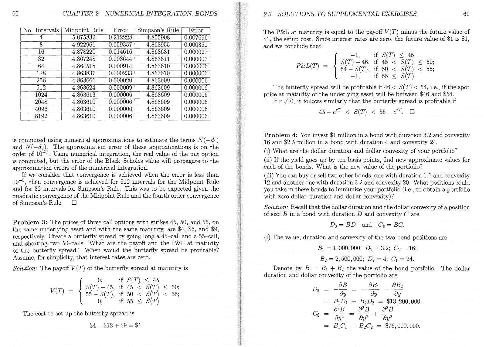
The
P&L
at
maturity
is equal
to
the
payoff
V(T)
minus
the
future value of
$1
,
the
setup cost. Since interest rates are zero,
the
future value of
$1
is
$1
,
and
we
conclude
that
(
-1
, if
S(T)
三
45;
PU(T)={:jTJfii;:35;
二::;
l
-1
, if
55
三
S(T)
The
b
时
terfly
spread will
be
pro
主
table
if
46
<
S(T)
<
54
, i.e., if
the
spot
price
at
maturity
of
the
underlying asset will be between
$46
and
$54.
If
r
并
0
,
it
follows similarly
that
the
butterfly spread is
pr
。在
table
if
45
+
erT
<
S(T)
<
55
-
erT
口
60
CHAPTER
2.
NUIVIERICAL
INTEGRATION.
BONDS.
No. Intervals Midpoint Rule Error
Simpson's Rule
Error
4 5.075832 0.212228
4.855908
0.007696
8
4.922961
0.059357 4.863955
0.000351
16 4.878220 0.014616 4.863631
0.000027
32 4.867248 0.003644 4.863611
0.000007
64 4.864518 0.000914 4.863610
0.000006
128 4.863837 0.000233
4.863610
0.000006
256 4.863666 0.000020 4.863609
0.000006
512 4.863624 0.000009 4.863609
0.000006
1024 4.863613 0.000006 4.863609
0.000006
2048 4.863610 0.000006 4.863609
0.000006
4096 4.863610 0.000006 4.863609
0.000006
8192 4.863610 0.000006 4.863609
0.000006
2.3.
SOLUTIONS
TO
SUPPLEMENTAL
EXERCISES
61
is computed
usi
吨
numerical
approximations
to
estimate
the
terms
N(
-d
1
)
and
N(
-d
2
)
工
The
approximation error of these approximations is
on
the
order of
10-
f
•
Using numerical integration,
the
real value of
the
put
option
is computed
,
but
the
error of
the
Black-Scholes value will propagate
to
the
approximation errors of
the
numerical integration.
If
we
consider
that
convergence
is
achieved when
the
error is less
than
10-
5
,
then
convergence is achieved for 512 intervals for
the
Midpoint Rule
and
for
32
intervals for Simpson's Rule. This was
to
be
expected given
the
quadratic convergence of
the
Midpoint Rule
and
the
fourth order convergence
of Simpson's
Rule.
口
Problem
3:
The
prices of
three
call options with strikes
45
,
50
, and
55
,
0
日
the
same underlying asset
and
with
the
same
maturity
, are
$4
,
$6
,
and
$9
,
respectively. Create a butterfly spread by going long a 45-call
and
a 55-call,
and
shorting two 50-calls.
What
are
the
payoff
and
the
P
&L
at
maturity
of
the
butterfly spread?
When
would
the
butterfly spread
be
profitable?
Assume
,for simplicity,
that
interest rates are zero.
Solution:
The
payoff
V(T)
of
the
butterfly spread
at
maturity
is
( 0
, if
S(T)
三
45;
J
S(T)
-
45
, if
45
<
S(T)
三
50;
V(T)=i55-S(TL
if50<S(T)<
吮
l 0, if
55
三
S(T).
The
cost
to
set up
the
butterfly spread is
$4 - $12
+
$9
=
$1.
Problem
4: You invest
$1
million in a bond with duration 3.2 and convexity
16
and
$2.5 million in a bond with duration 4
and
convexity
24.
(i)
What
are
the
dollar duration
and
dollar convexity of your portfolio?
(ii)
If
the
yield goes up by
ten
basis
points
,五nd
new approximate values for
each of
the
bonds.
What
is
the
new value of
the
portfolio?
(iii) You can buy or sell two
other
bonds,one with
duration
1.
6
and
convexity
12
and another one with duration 3.2
and
convexity
20.
What
positions could
you take in these bonds
to
immur
山
e
your portfolio (i.e.,
to
obtain
a portfolio
with zero dollar
duration
and dollar
co
盯
exity)?
Solution: Recall
that
the
dollar duration and
the
dollar convexity ofa position
of size
B in a bond with duration D and convexity
Care
D$
=
BD
and
C$
=
BC.
(i)
The
value, duration
and
co
盯
exity
of
the
two bond positions are
B
1
= 1,000,000; D
1
= 3.2; C
1
=
16;
B
2
= 2,
500
,000; D
2
=
4;
C
1
=
24.
Denote by
B
工
B
1
+ B
2
the
value of
the
bond portfolio.
The
dollar
duration
and
dollar convexity of
the
portfolio are
D
虫=一坐立一旦一
θ
B
2
ψθuθuθU
B
1
D
1
+ B
2
D
2
- $13,200,000.
C
虫
=θ
2B
θ2B+θ2β
川一一一
eθν2θν2θν2
B
1
C
1
+ B
2
C
2
- $76,000,000.

The
system (2.17) has solution B
3
= $3.25mil
and
B
4
=
-5.75mi
l.
We conclude
that
,
to
imm
飞
lnize
your portfolio, one should buy $3.25 mil-
lion worth of
the
bond with duration
1.
6
and
convexity
12
and
sell $5.75
million worth of
the
bond with duration
3.2
创
ld
convexity
20.
口
Formula (2.16) also holds for bond portfolios, since
the
dollar duration
and
the
dollar convexity of a bond portfolio are equal
to
the
sum of
the
dollar
duratioIIs azld of
th
dollar convexities of
the
bOIlds making
up
the
portfolio7
respectively.
Using (2.16)
,
we
五 nd
that
the
new value of
the
bond portfolio is
B
ne
ω
= B
十
i:::..
B 臼
$3
,
500
,
000
一
$13
,
200
十
$38
二
$3
,
486
,
838.
E[X]
=
汇
P(x
,
y)X(x
,
y)
=
去
L
X(x
,
y)
(X
,Y)ES
(x
,
y)
εS
63
If
2
三
k
~二
7
,
then
x + y = k if
and
only if
(x
,
y)
ε{(1
,
k -
1)
,
(2
,k -
2)
,… ,
(k
- 1,1)}.
In other words
,
x
十
y
= k for exactly k - 1 of
the
total
of
36
outcomes from
S.
Then
,
Chapter
3
Probability
concepts.
Black-Scholes
formula.
Greeks
and
Hedging.
3.1
Solutions
to
Chapter
3
Exercises
Problem
1:
Let k be a positive integer with
2
三
k
三
12.
You throw two
fair dice.
If
the
sum
of
the
dice
is
k,you win w(k
),
or lose 1 otherwise.
Find
the
smallest value of
ω
(k)
thats
makes
the
game worth playing.
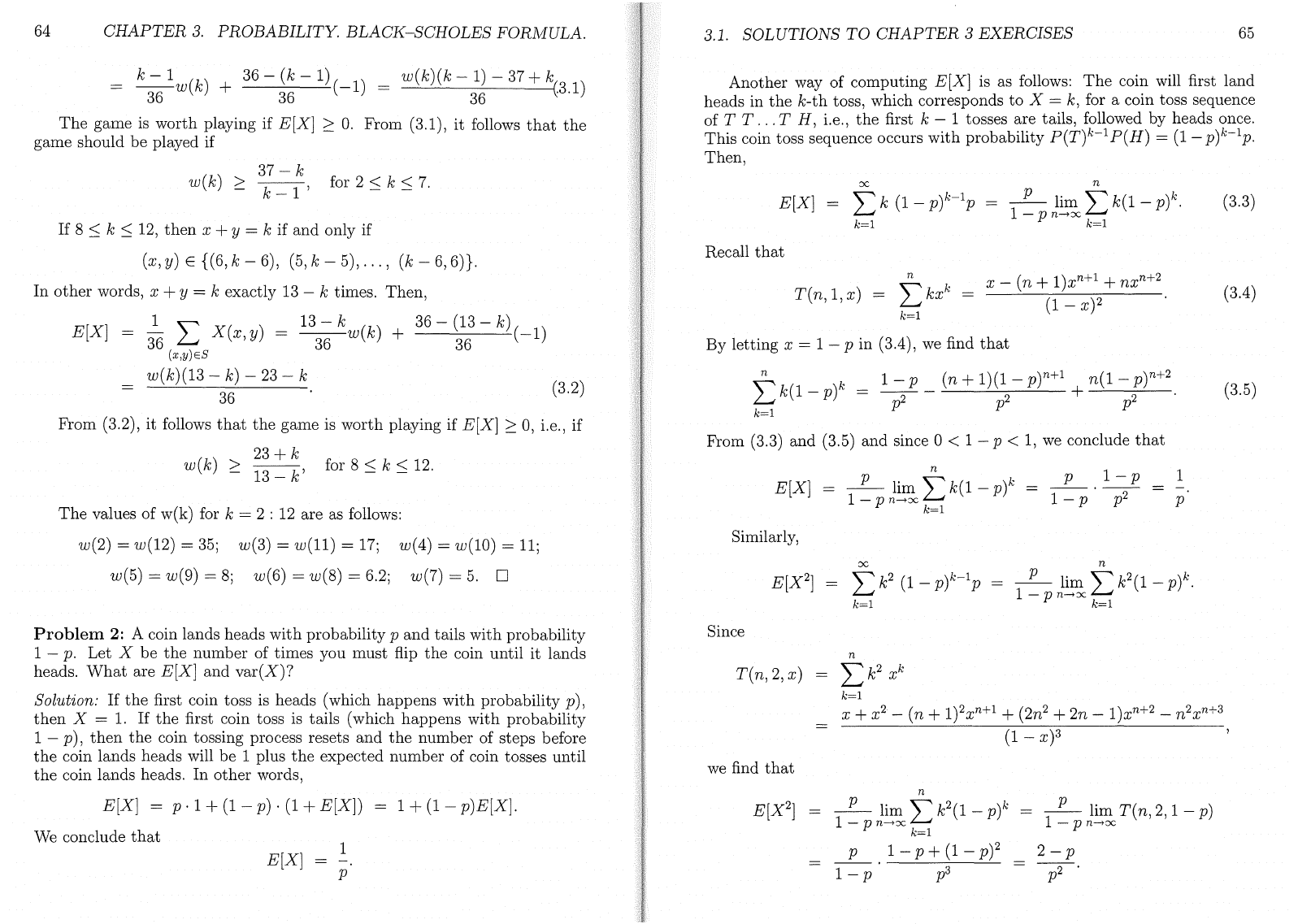
Solution: Consider
the
probability space S of all possible outcomes of throw-
ing of
the
two dice, i.e.,
S = {(x,y) I
x
二
1
: 6, y = 1 : 6}.
Here
, x
and
y denote
the
outcomes of
the
first
and
second die, respectively.
Since
the
dice are assumed
to
be
fair and
the
tosses are assumed
to
be inde-
pendent of each
other
, every outcome
(x
,
y)
且
as
probability
去
of
occurring
Formally
,
the
discrete probability function P : S •
[0
,
1]
is
P(x,
y)
=
二
,
V(x
,
y)
εS
36
Let
k be a fixed positive integer with 2
~二
k
~二
12.
The
value X of your
winning (or losses) is
the
random variable X : S
→~
given by
J w(k), if
x
十
y
=
k;
X(
川)巳
i-17else
(2.16)
(2.17)
CHAPTER
2.
NUMERICAL
INTEGRATION.
BONDS.
62
(ii) Using dollar duration
and
dollar
co
盯
exity
,
the
approximate formula
i:::..
B 1
7
倡一
-
D
i:::..
y + §C(
i:::..
y?
for
the
change in
the
value of a
bond
ca
丑
be
written
as
i:::..
B 臼
-D
向十
;C$(AU)2
(iii) Let B3 and B
4
be
the
value of
the
positions taken
i
口
the
bond
with
duration D
3
=
1.
6 and convexity C
3
-
12
and
in
the
bond
with
duration
D
4
= 3.2
and
convexity C
4
=
20
, respectively.
If
II = B +
B
3
十
B
4
denotes
the
value of
the
new portfolio,
the
丑
D$(II)
=
D$(B)
+
D$(B
3
)
+
D$(B
4
)
$13.2mil +
D
3
B
3
十
D
4
B
4
;
C$(
口)
=
D$(B)
+
D$(B
3
)
+
D$(B
4
)
$76mil +
C
3
B
3
十
C
4
B
4
.
Then
,
D$(
口)
= °
and
C$
(II) = °if
and
only if
(mml
十1.
6
川
2B
4
-
0;
$76mil + 12B
3
+
20
马-
0,
64
CHAPTER
3.
PROBABILITY.
BLACK-SCHOLES
FORl\/fULA.
k-l
36
一
(k
-
1)
一
ω
(k)(k
-
1)
- 37 + k
=丁百一
ω
(k)
十
~~
~/
(-1) _
~\'U/\'U
;~
VI
I
1~(3.1)
The
game is worth playing if
E[X]
三
O.
From (3.1),
it
follows
出
at
the
game should be played if
37 -
k
ω
(k)
兰一一
oj'
for 2
::;
k
::;
7.
k-l
If
8
~二
k
三
12
,
then
x
十
y
= k if
and
only if
(x
,
y)
ε
{(6
,
k-6)
,
(5
,
k-5)
,… , (k - 6,6)}.
In
other
words, x
十
y
= k exactly
13
- k times.
Then
,
E[X]
=
去汇
X(x
,
y)
=
与生
ω
(k)
十
36-T-k)(
一
1)
(x
,
y)
εS
ω
(k)(13-k)-23-k
36
From (3.2),
it
follows
that
the
game is worth
playi
吨
if
E[X]
三
0
,
i.e.,if
23+
k
ω
(k)
三一一"
for
8
三
k
< 12.
13
- k
(3.2)
The
values of w(k) for k = 2 : 12 are as follows:
ω(2)
=ω(12)
=
35;ω(3)
=ω(11)=17;ω(4)
=ω(10)
=
11;
ω(5)
=ω(9)
=
8;ω(6)
=ω(8)
=
6.2;ω(7)
=
5.
口
Problem
2: A coin lands heads
with
probability p
and
tails with probability
1 -
p. Let X
be
the
number of times you
lllUSt
flip
the
coin until it lands
heads.
What
are E[X] and
var(X)?
Sol
毗
on:
If
the
自
rst
coin toss is heads (which happens
with
probability
p)
,
then
X =
1.
If
the
自
rst
coin toss is tails (which happens with probability
1 -
p)
,
then
the
coin tossing process resets
and
the
number of steps before
the
coin lands heads will be 1 plus
the
expected number of coin tosses until
the
coin lands heads. In other words,
E
[X]
=
p'
1 +
(1
-
p)
.
(1
十
E[X])
= 1 +
(1-
p)E[X].
We conclude
that
1-P
X
E
3.1.
SOLUTIONS
TO
CHAPTER
3
EXERCISES
65
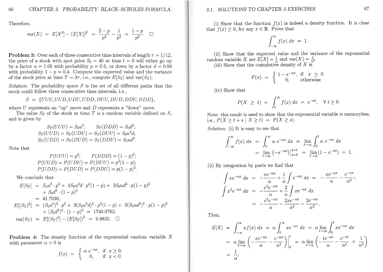
Another way of computing E[X] is as follows:
The
coin will first land
heads in
the
k-th toss,which corresponds
to
X = k,for a coin toss sequence
of
T
T.
..T H , i.
e.
,
the
first k - 1 tosses are tails, followed by heads once.
This
c
。如
toss
sequence occurs with probability
P(T)
川
P(H)
=
(1
- p)k-l
p
.
The
凡
E[X] L k
(1
- p)k-l
p
= 1
~?')
1~
L k(1 - p)k
品
pn
→
χ
仨?
(3.3)
Recall
that
T(
η
,
1
,
x)
(3
.4)
+-
n-
z-
1i-41i
/,,‘\-
By letting x = 1 - p
i
口
(3
.4),
we
直
nd
that
立
k
17P
(η
十川
_
p)n+l
I n(1 _
p)n+2
k(l-p)
fC
=
τ
了一
(3.5)
From (3.3) and (3.5)
and
since 0 < 1 - p < 1,
we
conclude
that
"ι
公
p
1-
p 1
E[X] =
~
lim)
~k(l-p)
日:一一
·-r=
一.
-pn
→
χ
仨
71-p
y p
Similarly,
E[X
2
]
L
对
(1
_
p)k-l
p
二
1
~?')nl~~Lk2(I-p)k
1-
pn
→
χ
仨?
Since
T(
η
,
2
,
x)
三二
k
2
x
k
X
+x
2
一
(n
十
1)2
x
n+l
+
(2η2
十
2η
-
l)x
n
+
2
一
η
2
X
n
十
3
(1
x)3
we
find
that
E[X
2
]
n
..
p _ lim
~
k
2
(1-
p)k =
~
lim
T(n
,2,1 -
p)
仨
71-pn
→∞
pl
… p +
(1
-
p)2
1-
P
p3
2-p
2
p
66
CHAPTER
3.
PROBABILITY.
BLACK-SCHOLES
FORNIULA.
Therefore,
var(X)
=
E[X
2
]
一
(E[X])2
2 - p 1
p2
p2
匕主口
P'"
Problem
3:
Over each of
three
consecutive
time
i
时
ervals
ofle
丑
gth
7 =
1/12
,
the
price of a stock
with
spot
price 8
0
= 40
at
time
t = 0 will either go
up
by a factor u =
1.
05
with
probability p = 0.6,
or
down by a factor d = 0.96
with
probability 1 - p = 0
.4.
Compute
the
expected value
and
the
variance
of
the
stock price
at
time
T = 37,i.e.,
compute
E[8
T
]
and
var(8
T
).
Solution:
The
probability space 8 is
the
set of all different
paths
that
the
stock could follow
three
consecutive
time
intervals,i.e. ,
8 = {UUU,UUD,UDU,
UDD
,
DUU
,
DUD
,
DDU
,
DDD}
,
where U represents
an
"up" move
and
D represents a "down" move.
The
value 8
T
of
the
stock
at
time
T is a
random
variable
de
五日
ed
on
8 ,
and
is given by
8T(UUU)
二
S
旷
;
8
T
(DDD)
= 8
0
d
3
;
8
T
(UUD)
= 8
T
(UDU) = 8T(DUU) = 8
0
u
2
d;
8
T
(UDD) = 8
T
(DUD) = 8
T
(DDU) = 8
0
ud
2
.
Note
that
P(UUU) =
p3;
P(DDD)
=
(1
_
p)3;
P(UUD) = P(UDU) =
P(DUU)
=
p2(1_
p);
P(UDD)
=
P(DUD)
=
P(DDU)
=
p(l-
p?
We conclude
that
E[8T]
80u3
.
p3
十
38
0
饥
2d.p2(1_p)+
38
0
叫
2
.
p(l
_
p)2
十
8
0
d
3
.
(1
_
p)3
4
1.
7036;
但
OU
3
)2
.
p3
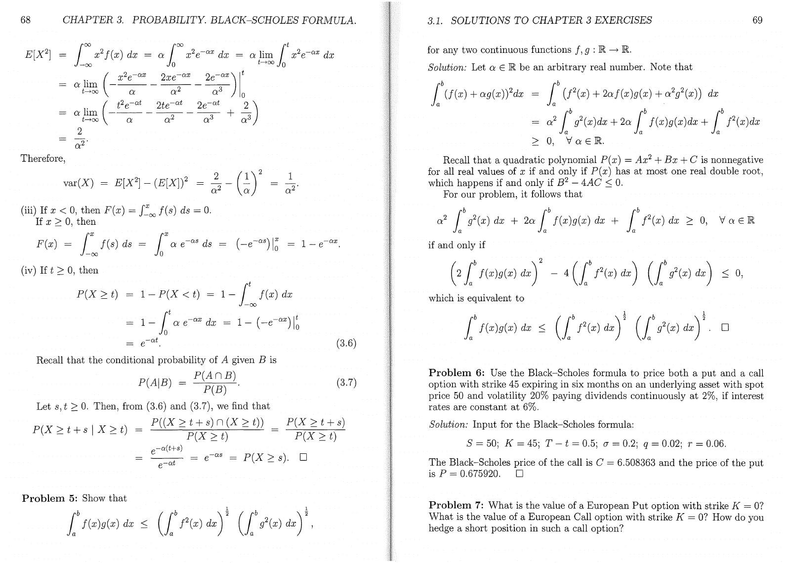
+
3(8
0
u
2
d)2.
p2(1
-
p)
+
3(8
0
ud
2
)2.
p(l
_
p)2
十
(8
0
d
3
)2
. (1 -
p)3
= 1749.0762;
E[(8T
)2]
一
(E[8T])2
工
9.8835.
口
E[(8
T
)2]
var(8
T
)
Problem
4:
The
density function of
the
exponential
random
variable X
with
parameterα>
0 is
J a
e
一
αzif
Z > 0;
f(x)
=
)、
77if
Z
二。
3.1. SOLUTIONS
TO
CHAPTER
3
EXERCISES
67
(i) Show
that
the
function
f(x)
is indeed a density function.
It
is clear
that
f(x)
三
0
,
for any x
εJR.
Prove
that
汇
f
川=
1
(ii) Show
tl
时
the
expected value
and
the
variance of
the
expo
阳
rando
'm
variable X are E[X] = i
and
var(X)
=去
(iii) Show
that
the
cumulative
de
丑
sity
of X is
r
1-
e
一
α
x
if x > 0
F(x)
=
γ0770
阳飞
Nis
(iv) Show
that
M
三
t)
=
f
川
x
=
川
Vt
主
O
Note: this result is used
to
show
that
the
exponential variable is memoryless,
i.e.,
P(X
三
t
十
s
I
X
三
t)
=
P(X
三
s
).
Sol
础。即
(i)
It
is easy
to
see
that
汇
f
川
fα
川
z=J
叫
tα
川
Z
出
(-rz)lZ
Z
出
(1
-
e
一叫
= 1
(ii) By integration by
parts
we
find
that
J
xe
叫
z
f
泸川
Z
xe
一
α
x
1 r
~_嘈
一一一一一+…
I
e-
Uw
dx
ααl
一生主+~
r
xe
一
ω
dx
ααl
x
2
e
一
α
x
2xe
一
α
x
2e
一
αz
αα2α3
一
α
x
~一
α
x
xe
--
e
αα2
'
1-d
d
pu
z-
fl04-g
etnu
z--iii
z-
rJ
'ME
T
α
68
CHAPTER
3.
PROBABILITY.
BLACK-SCHOLES
FORJYIULA.
3.1.
SOLUTIONS
TO
CHAPTER
3
EXERCISES
69
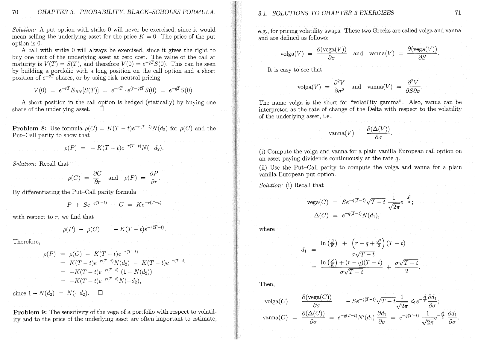
E[X
2
]
LW)dz=due-α
♂
dx
工
αEtjtpzdz
叫一午一平
_
2~3ax)
I:
αJ
坦(一午
-25ff-23+
主)
1-e
一
α
X
for
any
two
continuous
functions
f
,
g :
JR
•
JR.
Solution:
Let
αεJR
be
an
arbitrary
real number. Note
that
l
ρb
飞
U(υ
f(
叫川+忖
α
以仰州
Z
叫
ω
巾)川)
α
21
b
g2(x)dx
+
叫
b
仲州川
)g
川
g
~
0
,
V
αεJR.
Recall
that
a
quadratic
polynomial
P(
x)
=
Ax
2
十
Bx
+
C is nonnegative
for all real values
of
x
if
and
only if P(x)
has
at
most
one real
double
root
,
which
happens
if
and
only
if
B
2
-
4AC
三
O.
For
our
problem
,
it
follows
that
α2
l
b
9"
川+叫
bf(Z)g(Z)dz+ff2
川三
0
,
VαεR
if
and
only
if
Therefore
var
叫叫
a
町叫州
r
刘伊帆(仪问
X
刻)
=
州
一
(但
E[X
啊[阿冈附
X
判]
(仙
i
拄
i
垃
i)
1f
x
<
0
,
then
F(x)
=
J~
∞
f(s)
ds
=
O.
1f
x
主
0
,
the
口
咐:汇川
s
=
fa"
αf
叫
=
(-e-
α
s)
I~
(iv)
1f
t
三
0
,
then
1
α2
P(X
主
t)
1-
P(X
<
t)
=
1
一
λρ
扣
f
只(阳
Z
叫州)川
d
l
一l'
αω
巳一叫
=
1
一
(-e
ω)
I~
nu
\IlI-
,/
Z
z
nL
'O
/II--\
z
Z
rId
LU
/Il--\
\Ill-/
Z
,
G
Z
ny
z
rId
,
/lil\
which is
equivalent
to
(3.6)
z
Z
od
Thu
/It--\
Z
JU
z
n
,,"
rld
-o
/III-\
<-
2
,
G
ZZ
J'i\
rId
'D
P(X
主
t+s
I
X
三
t)
Recall
that
the
conditional
probability
of A
given
B is
P(A
n
B)
P(AIB)
=
P(B)
Let
s
,
t
三
O.
The
凡
from
(3.6)
and
(3.7)
,
we find
that
P((X
三
t+s)n(x
主
t))
P(X
三
t
+
s)
P(X
三
t)
P(X
三
t)
e
一
α
(
t+
s)
_,""
If
工
e
一讪-甲-
ε'-'0
(3.7)
Problem
6:
Use
the
Black-Scholes
formula
to
price
both
a
put
and
a call
option
wit
且
strike
45 expiring
in
six
months
on
an
underlying
asset
with
spot
price
50
and
volatility 20%
paying
dividends
continuously
at
2%
,
if
interest
rates
are
constant
at
6%.
Solution:
Input
for
the
Black-Scholes
formula:
S
=
50;
K
=
45;
T
-
t
=
0.5;σ=
0.2;
q
=
0.02;
r
=
0.06.
The
Black-Scholes
price
of
the
call is
C
=
6.508363
and
the
price of
the
put
is P
=
0.675920.
口
l
f(x)g(
川三
(l
尸
(x)
dx
)'
(l
g2
川)\
Problem
7:
What
is
the
value
of
a
European
Put
option
with
strike
K
=
07
毛iV
hat
is
the
value of
a
European
Call
option
with
strike
K
=
07
How
do you
hedge
a
short
position
in such a call
option
7
70
CHAPTER
3.
PROBABILITY.
BLACK-SCHOLES
FORNIULA.
3.1.
SOLUTIONS
TO
CHAPTER
3
EXERCISES
71
Solution: A
put
option with strike 0 will never
be
exercised, since
it
would
mean selling
the
underlying asset for
the
price K =
O.
The
price of
the
put
option is
O.
A call
with
strike 0 will always be exercised, since
it
gives
the
right
to
buy
one
u
日
it
of
the
underlying asset
at
zero cost.
The
value of
the
call
at
maturity
is
V(T)
工
8(T)
,
and
therefore
V(O)
工
e-
qT
8(0). This can
be
seen
by building a portfolio with a long position on
the
call option and a short
position of
e-
qT
shares,or by using
risk-neutral
pricing:
V(O)
e-
rT
E
RN
[8(T)]
e-
rT
.
e(r
一伊
8(0)
二
e-
qT
8(0).
A short position i
口
the
call
optior
丑
1
1
祀
s
hedged
(s
剖
ta
创
tic
伪
a
址
11
与坊圳
y
吵
7
→)
by buying
0
∞
l
口
1
share of
the
underlying
asset.
口
e.g.,for pricing volatility swaps. These two Greeks are called volga
and
vanna
and are
de
如
led
as follows:
θ(vega(V))θ(vega(V))
volga(V)
=θσand
vanna(V)
=θS
It
is easy
to
see
that
θ
2V
θ
2V
volga(V)
=万万
and
vanna(V)
-否瓦
The
name volga is
the
short for "volatility gamma". Also, vanna can
be
interpreted as
the
rate
of change of
the
Delta
with
respect
to
the
volatility
of
the
underlying asset,i.e.,
(i) Compute
the
volga
and
vanna for a
plai
丑
vanilla
European call option on
an
asset paying dividends continuously
at
the
rate
q.
(ii) Use
the
Put-Call
parity
to
compute
the
volga
and
vanna for a plain
vanilla European
put
option.
Solution: (i) Recall
that
vanna(V)
Problem
8: Use formula p(
C)
=
K(T
-
t)e-r(T-t)
N(
也)
for p(C)
and
the
Put-Call
parity
to
show
that
p(P)
= -
K(T
-
t)e-r(T-t)
N(-d
2
).
Solution: Recall
that
θCθP
p(C)
=
a~
and
p(P)
=
万;
By differentiating
the
Put-Call
parity
formula
P +
8e-
q
(T-t)
- C K e-r(T-t)
with
respect
to
飞
we
find
that
p(P)
-
p(C)
=
-K(T-t)e-r(T-t).
where
vega(C)
~(C)
θ
(~(V))
θσ
8e-
q
(T-t)
叮叮
-LJ:
飞
/27
了'
e-q(T-t)
N(d
1
)
,
θ(
吵
(C))
_
-
8e-
q
(T-t
哺可
-L
dJf11;
Uσ
飞
/2
7r
-
d
σ'
θ
(~(C))_
e-q(T-t)
N'(d
1
)
纽
-
e-
q
叫↓
λ
ad
1
θσ
〉三作
θσ
Therefore,
p(P)
=
ρ
(C)
-
K(T
-
t)e-r(T-t)
K(T
-
t)e-r(T-t)
N(d
2
)
-
K(T
-
t)e-r(T-t)
-K(T
-
t)e-r(T-t)
(1
-
N(d
2
))
-
K(T
-
t)e-r(T-t)
N(
-d
2
)
,
since 1 -
N(d
2
) =
N(-d
2
).
口
Problem
9:
The
sensitivity of
the
vega of a portfolio
with
respect
to
volatil-
ity
and
to
the
price of
the
underlying asset are often
important
to
estimate,
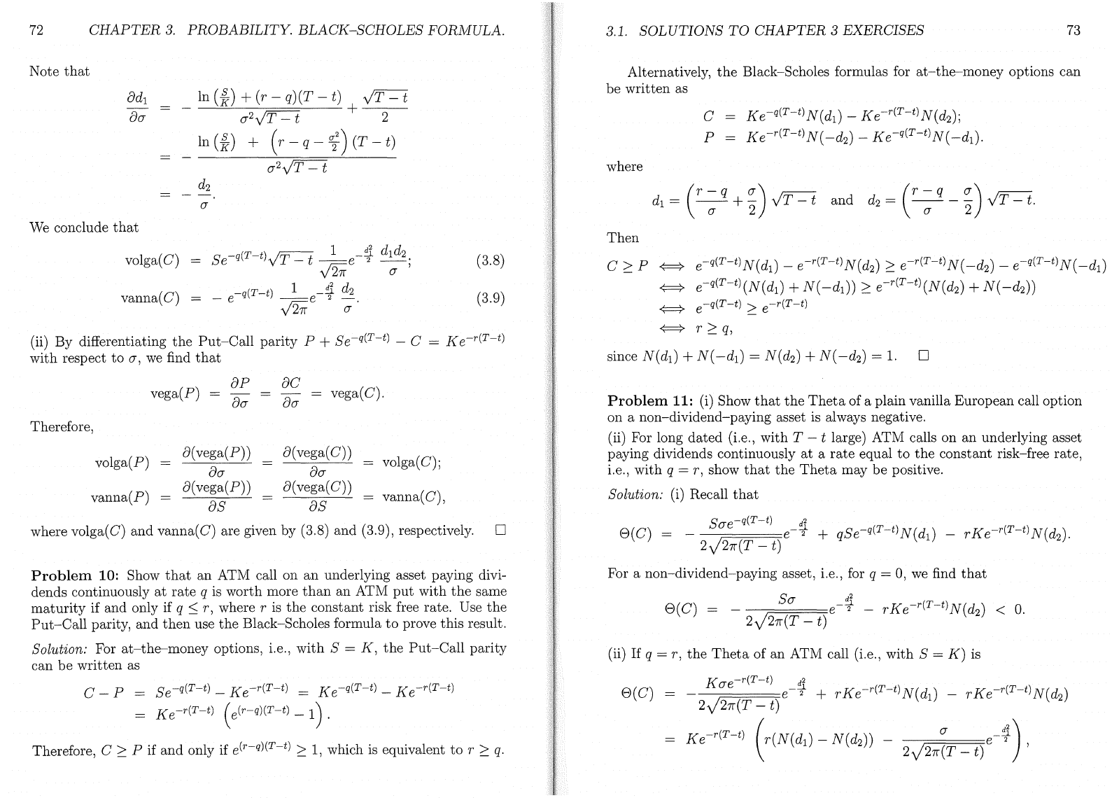
Then
,
volga(C)
vanna(C)
d
1
叶
)
+
(γ
-q
吟)
(T
- t)
VT
丁
Z
In
(去)
+
(r
… q)(T -
t)
tσ
VTτz
σ
VT
丁
t
2
72
CHAPTER
3.
PROBABILITY.
BLACK-SCHOLES
FOR~
在
ULA.
3.1.
SOLUTIONS
TO
CHAPTER
3
EXERCISES
73
(ii) By differentiating
the
Put-Call
parity
P
十
Se-q(T-t)
- C = K e-r(T-t)
with
respect
to
风
we
find
that
Note
that
θ
d
1
θσ
We conclude
that
volga(C)
vanna(C)
In
(圣)
+
(γ
-
q)(T
-
t)
,~丁
I
一二
σ2VT
士
t
2
叫)
+
(γ
-q
一手)
(T
-
t)
σ2
飞厅可
d
2
σ
Se-
旷
-tL
.j
T
丁
zi-e
千生生
川
νd
开
σ7
-e-q(T-t)
」
-e-4d2
d
石
σ
(3.8)
(3.9)
Alternatively
,
the
Black-Scholes formulas for
at-th
e-
money options can
be written as
C -
Ke-q(T-t)
N(d
1
) -
Ke-r(T-t)
N(
出);
P -
Ke-
r
(T-t)N(-d
2
) -
Ke-
q
(T-t)N(-d
1
).
where
叶子气)旧
and
叫于一~)旧
Then
C
三
P
仁=?
e-q(T-t)
N(d
I)
- e-r(T-t)
N(d
2
)
三
e-r(T-t)
N(
-d
2
) -
e-q(T-t)
N(
-d
1
)
中=争
e
一旷一气
N(d
1
)
+
N(
-d
1
))
三
e-r(T
一气
N(d
2
)
+
N(
-d
2
))
牛=辛
>
e-q(T-t) > e-r(T-t)
牛=学
γ
二三
q,
since
N(d
1
) +
N(
-d
1
) =
N(d
2
) +
N(
-d
2
) =
1.口
θ(vega(P))θ(vega(C))
Volga(P)z
=z
Volga(C);
θσθσ
θ(vega(P))θ(vega(C))
vama(P)===vanm(C)?
θSθs
where volga(C)
and
van
叫
C)
are given by (3.8)
and
(3.9),respectively.
Therefore
,
θP
vega(P) -
否歹
δC
歹歹工
vega(C).
口
Pro
blem
11:
(i) Show
that
the
Theta
of a plain vanilla
E
旧
opean
call option
on a non-dividend-paying asset is always negative.
(ii) For long
dated
(i.e., with T - t large)
ATJVI
calls on an underlying asset
paying dividends continuously
at
a
rate
equal
to
the
constant risk-free
rate
,
i.e., with q = r , show
that
the
Theta
may
be
positive.
Solution:
(i)
丑
ecall
that
Sσ
e-q(T-t)
~
@(C)=-e
2
十
qSe-q(T-t)
N(d
1
) -
rK e-r(T-t)
N(d
2
).
2 、
/2π(T
- t)
Problem
10: Show
that
an
ATM call on
an
underlying asset paying divi-
dends continuously
at
rate
q is worth more
than
an
ATM
put
with
the
same
maturity
if and only if
q
三飞
where
r is
the
constant risk free rate. Use
the
Put-Call
parity,
and
then
use
the
Black-Scholes formula
to
prove this result.
Solution: For
at-th
e-
money options, i.e.,
with
S = K ,
the
Put-Call
parity
can
be
written
as
C - P = Se-q(T-t) - K e-r(T-t) _ K e-q(T-t) - K e-r(T-t)
K e-r(T-t) (e(r-q)(T-t) -
1)
Therefore, C
~三
P
if
and
only if e(r-q)(T-t)
;
三
1
,
which is equivalent
to
r
主
q.
For a non-dividend-paying asset,i.e., for q = 0,
we
find
that
8(C)
=
-Sσe-4-Tke-r(T-t)N(d2)<0.
2 飞
/2
作
(T
-
t)
(ii)
If
q = r ,
the
Theta
of an ATM call (i.e.,
with
S =
K)
is
Kae-r(T-t)
-~
@(C)=-e2
十
r
K e-r(T-t)
N(
d
1
) -
rK e-r(T-t)
N(
d
2
)
2 飞
/2
作
(T
-
t)
Ke-r(T-t)
(r(N(d
1
) -
N(d
2
))
一
σJ)
\2
飞
/2
汀
(T
-
tr
)
