Soong T.T. Fundamentals of Probability and Statistics for Engineers
Подождите немного. Документ загружается.

and (11.23) with the Cram r–Rao lower bounds defined in Section 9.2.2. In
order to evaluate these lower bounds, a probability distribution of Y must be
made available. Without this knowledge, however, we can still show, in Theorem
11.2, that the least squares technique leads to linear unbiased minimum-variance
estimators for and ; that is, among all unbiased estimators which are linear
in Y , least-square estimators have minimum variance.
Theorem 11.2: let random variable Y be defined by Equation (11.4). Given
asample(x
1
,Y
1
), (x
2
,Y
2
), . . . , (x
n
,Y
n
) of Y with its associated x values, least-
given by Equation (11.17) are minimum variance
linear unbiased
estimators
for and , respectively.
Proof of Theorem 11.2: the proof of this important theorem is sketched
below with use of vector–matrix notation.
Consider a linear unbiased estimator of the form
We thus wish to prove that G 0 if
*
is to be minimum variance.
The unbiasedness requirement leads to, in view of Equation (11.19),
Consider now the covariance matrix
Upon using Equations (11.19), (11.24), and (11.25) and expanding the covari-
ance, we have
Now, in order to minimize the variances associated with the components of
,
we must minimize each diagonal element of GG
T
. Since the iith diagonal
element of GG
T
is given by
where g
ij
is the ijth element of G, we must have
and we obtain
344
Fundamentals of Probability and Statistics for Engineers
square estimators and
Â
^
A
^
B
Q
*
C
T
C
1
C
T
GY: 11:24
Q
*
GC 0: 11:25
covfQ
*
gEfQ
*
qQ
*
q
T
g: 11:26
covfQ
*
g
2
C
T
C
1
GG
T
:
Q
*
GG
T
ii
X
n
j1
g
2
ij
;
g
ij
0; for all i and j:
G 0: 11:27
e
TLFeBOOK

This completes the proof. The theorem stated above is a special case of the
Gauss–Markov theorem.
Another interesting comparison is that between the least-square estimators
for and and their maximum likelihood estimators with an assigned dis-
tribution for random variable Y . It is left as an exercise to show that the
maximum likelihood estimators for and are identical to their least-square
counterparts under the added assumption that Y is normally distributed.
11.1.3 UNBIASED ESTIMATOR FOR
2
As we have shown, the method of least squares does not lead to an estimator
for variance
2
of Y , which is in general also an unknown quantity in linear
regression models. In order to propose an estimator for
2
, an intuitive choice is
where coefficient k is to be chosen so that
is unbiased. In order to carry out
the expectation of
, we note that [see Equation (11.7)]
Hence, it follows that
since [see Equation (11.8)]
Upon taking expectations term by term, we can show that
Linear Models and Linear Regression 345
c
2
k
X
n
i1
Y
i
^
A
^
Bx
i
2
; 11:28
c
c
Y
i
^
A
^
Bx
i
Y
i
Y
^
Bx
^
Bx
i
Y
i
Y
^
Bx
i
x:
11:29
X
n
i1
Y
i
^
A
^
Bx
i
2
X
n
i1
Y
i
Y
2
^
B
2
X
n
i1
x
i
x
2
; 11:30
X
n
i1
x
i
xY
i
Y
^
B
X
n
i1
x
i
x
2
: 11:31
Ef
c
2
gkE
X
n
i1
Y
i
Y
2
^
B
2
X
n
i1
x
i
x
2
()
kn 2
2
:
2
2
TLFeBOOK

Hence,
2
is unbiased with k 1/(n 2), giving
or, in view of Equation (11.30),
Example 11.2. Problem: use the results given in Example 11.1 and determine
an unbiased estimate for
2
.
Answer: we have found in Example 11.1 that
In addition, we easily obtain
Equation (11.33) thus gives
Example 11.3. Problem: an experiment on lung tissue elasticity as a function
of lung expansion properties is performed, and the measurements given in
Table 11.2 are those of the tissue’s Young’s modulus (Y ), in gcm
2
,atvarying
values of lung expansion in terms of stress (x), in gcm
2
. Assuming that E Y
is linearly related to x and that
2
Y
2
(a constant), determine the least-square
estimates of the regression coefficients and an unbiased estimate of
2
.
Table 11.2 Young’s modulus, y (gcm
2
), with stress, x (g cm
2
), for Example 11.3
x22.535791012151617181920
y 9.1 19.2 18.0 31.3 40.9 32.0 54.3 49.1 73.0 91.0 79.0 68.0 110.5 130.8
346 Fundamentals of Probability and Statistics for Engineers
c
c
2
1
n 2
X
n
i1
Y
i
^
A
^
Bx
i
2
; 11:32
c
2
1
n 2
X
n
i1
Y
i
Y
2
^
B
2
X
n
i1
x
i
x
2
"#
: 11:33
X
n
i1
x
i
x
2
2062:5;
^
0:57:
X
n
i1
y
i
y
2
680:5:
b
2
1
8
680:5 0:57
2
2062:5
1:30:
f g
TLFeBOOK

Answer: in this case, we have n 14. The quantities of interest are
The substitution of these values into Equations (11.7), (11.8), and (11.33) gives
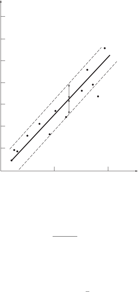
The estimated regression line together with the data are shown in Figure 11.3.
The estimated standard deviation is 13 g cm
2
,andthe
1 -band is also shown in the figure.
11.1.4 CONFIDENCE INTERVALS FOR REGRESSION
COEFFICIENTS
In addition to point estimators for the slope and intercept in linear regression, it
is also easy to construct confidence intervals for them and for x, the mean
of Y , under certain distributional assumptions. In what follows, let us assume
that Y is normally distributed according to N( x,
2
). Since estimators
and x are linear functions of the sample of Y , they are also normal
random variables. Let us note that, when sample size n is large, and
are expected to follow normal distributions as a consequence of the
central limit theorem (Section 7.2.1), no matter how Y is distributed.
We follow our development in Section 9.3.2 in establishing the desired
confidence limits. Based on our experience in Section 9.3.2, the following are
not difficult to verify:
Linear Models and Linear Regression 347
x
1
n
X
n
i1
x
i
1
14
2 2:5 2011:11;
y
1
n
X
n
i1
y
i
1
14
9:1 19:2 130:857:59;
X
n
i1
x
i
x
2
546:09;
X
n
i1
y
i
y
2
17; 179:54;
X
n
i1
x
i
xy
i
y2862:12:
^
2862:12
546:09
5:24;
^
57:59 5:2411:110:63;
b
2
1
12
17; 179:54 5:24
2
546:09 182:10:
^
p
2
,
^
A,
^
B
^
A
^
^
A,
^
B,
^
A
^
Bx
B
,
182:10 13 49 g cm
:
TLFeBOOK
.
Result i: let
2
be the unbiased estimator for
2
as defined by Equation
(11.33), and let
It follows from the results given in Section 9.3.2.3 that D is a
2
-distributed
random variable with (n 2) degrees of freedom.
.
Result ii: consider random variables
^
^
^^
y
=
+
x
10 20
0
20
40
60
80
100
120
140
Young's modulus,
y
(g/cm
2
)
Stress,
x
(g/cm
2
)
Figure 11.3 Estimated regression line and observed data, for Example 11.3
348 Fundamentals of Probability and Statistics for Engineers
c
D
n 2
c
2
2
: 11:34
^
A
c
2
X
n
i1
x
2
i
"#
n
X
n
i1
x
i
x
2
"#
1
8
<
:
9
=
;
1=2
; 11:35
σ
^
α β
σ
TLFeBOOK

and
where, as seen from Equations (11.20), (11.22), and (11.23), and are,
2
estimated by
2
. The derivation
given in Section 9.3.2.2 shows that each of these random variables has a
t-distribution with (n 2) degrees of freedom.
.
Result iii: estimator for the mean of Y is normally distributed with
mean x and variance
Hence, again following the derivation given in Section 9.3.2.2, random variable
is also t-distributed with (n 2) degrees of freedom.
Based on the results presented above, we can now easily establish confidence
limits for all the parameters of interest. The results given below are a direct
consequence of the development in Section 9.3.2.
.
Result 1: a [100(1 )]% confidence interval for is determined by [see
Equation (9.141)]
Linear Models and Linear Regression 349
respectively, the means of and and the denominators are, respectively,
the standard deviations of and with
^
B
c
2
X
n
i1
x
i
x
2
"#
1
8
<
:
9
=
;
1=2
11:36
^
A
^
B
^
A
^
B
c
EfYg
varf
d
EfYgg varf
^
A
^
Bxg
varf
^
Agx
2
varf
^
Bg2xcovf
^
A;
^
Bg
2
X
n
i1
x
i
x
2
"#
1
1
n
X
n
i1
x
2
i
x
2
2xx
!
2
1
n
x
x
2
X
n
i1
x
i
x
2
"#
1
8
<
:
9
=
;
:
11:37
d
EfYg x
hi
c
2
1
n
x
i
x
2
X
n
i1
x
i
x
2
"#
1
8
<
:
9
=
;
8
<
:
9
=
;
1=2
11:38
L
1;2
^
A t
n2;=2
c
2
X
n
i1
x
2
i
!
n
X
n
i1
x
i
x
2
"#
1
8
<
:
9
=
;
1=2
: 11:39
d
TLFeBOOK

.
Result 2: a [100(1 )% confidence interval for is determined by [see
Equation (9.141)]
.
Result 3: a [100(1 )]% confidence interval for E Y x is deter-
mined by [see Equation (9.141)]
.
Result 4: a two-sided [100(1 )% confidence interval for
2
is determined
by [see Equation (9.144)]
If a one-sided confidence interval for
2
is desired, it is given by [see Equation
(9.145)]
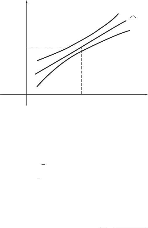
A number ofobservations can be made regarding these confidence intervals. In
each case, both the position and the width of the interval will vary from sample
to sample. In addition, the confidence interval for x is shown to be a
function of x. If one plots the observed values of L
1
and L
2
they form a
confidence band about the estimated regression line, as shown in Figure 11.4.
Equation (11.41) clearly shows that the narrowest point of the band occurs at
x
x; it becomes broader as x moves away from x in either direction.
Ex ample 11. 4. Problem: in Example 11.3, assuming that Y is normally
distributed, determine a 95% confidence band for
350
Fundamentals of Probability and Statistics for Engineers
L
1; 2
^
B t
n2;=2
c
2
X
n
i1
x
i
x
2
"#
1
8
<
:
9
=
;
1=2
: 11:40
f g
L
1;2
d
EfYgt
n2;=2
c
2
1
n
x
x
2
X
n
i1
x
i
x
2
"#
1
8
<
:
9
=
;
8
<
:
9
=
;
1=2
: 11:41
L
1
n 2
c
2
2
n2;=2
;
L
2
n 2
c
2
2
n2;1=2
:
11:42
L
1
n 2
c
2
2
n1;
:11:43
x.
TLFeBOOK
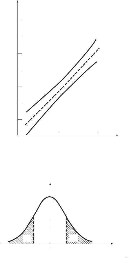
Answer: equation (11.41) gives the desired confidence limits, with n 14,
The observed confidence limits are thus given by
This result is shown graphically in Figure 11.5.
11.1.5 SIGNIFICANCE TESTS
Following the results given above, tests of hypotheses about the values of and
can be carried out based upon the approach discussed in Chapter 10. Let us
demonstrate the underlying ideas by testing hypothesis H
0
:
0
against
hypothesis H
1 0
,where
0
is some specified value.
y
x
x
+
^
^
(
x
)
l
2
(
x
)
l
1
x
+
E
(
y
) =
x
^
^
–
–
Figure 11.4 Confidence band for
Linear Models and Linear Regression
351
d
Efyg
^
^
x 0:63 5:24x;
t
n2;=2
t
12;0:025
2:179; from Table A.4;
x 11:11;
X
n
i1
x
i
x
2
546:09;
b
2
182:10:
l
1; 2
0:63 5:24x2:179 182:10
1
14
x 11:11
2
546:09
"#()
1=2
:
6
α β
β
EfYg x
:
α
0 05, and
:
TLFeBOOK
Using as the test statistic, we have shown in Section 11.1.4 that the random
variable defined by Equation (11.36) has a t-distribution with n 2 degrees of
freedom. Suppose we wish to achieve a Type-I error probability of . We would
reject H
0
if exceeds (see Figure 11.6)
0
10 20
20
40
60
80
100
120
140
x
+
^
(
x
)
l
2
(
x
)
l
1
Young’s modulus,
y
(g/cm
2
)
Stress,
x
(g/cm
2
)
^
Figure 11. 5 The 95% confidence band for E Y for Example 11.4
1–
/2
/2
–
t
n,
/2
t
n,
/2
f
T
(
t
)
t
Figure 11. 6 Probability density function of T
352 Fundamentals of Probability and Statistics for Engineers
^
B
j
^
0
j
α β
f g
γ
γ
γ
γ γ
(
^
B
0
)
c
2
[
P
n
i1
(x
i
x)
2
]
1
1/2
,
TLFeBOOK

Similarly, significance tests about the value of can be easily carried out with
use of as the test statistic.
An important special case of the above is the test of H
0
: 0 against
H
1
: 0. This particular situation corresponds essentially to the significance
test of linear regression. Accepting H
0
is equivalent to concluding that there is
no reason to accept a linear relationship between E Y and x at a specified
significance level . In many cases, this may indicate the lack of a causal
relationship between E Y and independent variable x.
Example 11.5. Problem: it is speculated that the starting salary of a clerk is a
function of the clerk’s height. Assume that salary (Y ) is normally distributed and
its mean is linearly related to height (x); use the data given in Table 11.3 to test
the assumption that E Y and x are linearly related at the 5% significance level.
Answer: in this case, we wish to test H
0
: 0 against H
1
0,with 0:05.
From the data in Table 11.3, we have
According to Equation (11.44), we have
Table 11. 3 Salary, y (in $10 000), with height, x (in feet),
for Example 11.5
x 5.7 5.7 5.7 5.7 6.1 6.1 6.1 6.1
y 2.25 2.10 1.90 1.95 2.40 1.95 2.10 2.25
Linear Models and Linear Regression
353
t
n2;=2
b
2
X
n
i1
x
i
x
2
"#
1
8
<
:
9
=
;
1=2
: 11:44
^
A
6
f g
f g
f g
: 6
^
X
n
i1
x
i
xy
i
y
"#
X
n
i1
x
i
x
2
"#
1
0:31;
t
n2;=2
t
6;0:025
2:447; from Table A.4;
b
2
1
n 2
X
n
i1
y
i
y
2
^
2
X
n
i1
x
i
x
2
"#
0:02;
X
n
i1
x
i
x
2
0:32:
t
6;0:025
b
2
X
n
i1
x
i
x
2
"#
1
8
<
:
9
=
;
1=2
0:61:
TLFeBOOK