Soong T.T. Fundamentals of Probability and Statistics for Engineers
Подождите немного. Документ загружается.


where
The theorems stated in this section do not apply in this case to the portions
v
1
<95Vandv
1
> 105V because infinite and noncountable number of roots
for v
1
exist in these regions. However, we deduce immediately from Figure 5.14
that
For the middle portion, Equation (5.7) leads to
Now,
We thus have
ThePDF, F
V
2
(v
2
), is shown in Figure 5.15, an example of a mixed distribution.
5.1.2 MOMENTS
Having developed methods of determining the probability distribution of
Y g(X), it is a straightforward matter to calculate all the desired moments
134
Fundamentals of Probability and Statistics for Engineers
gV
1
0; V
1
< 95;
gV
1
V
1
95
10
; 95 V
1
105;
gV
1
1; V
1
> 105:
PV
2
0PV
1
95F
V
1
95
Z
95
90
f
V
1
v
1
dv
1
1
4
;
PV
2
1PV
1
> 1051 F
V
1
105
1
4
:
F
V
2
v
2
F
V
1
g
1
v
2
F
V
1
10v
2
95; 0 < v
2
< 1:
F
V
1
v
1
v
1
90
20
; 90 v
1
110:
F
V
2
v
2
1
20
10v
2
95 90
2v
2
1
4
; 0 < v
2
< 1:
TLFeBOOK

of Y if they exist. However, this procedure – the determination of moments of Y
on finding the probability law of Y – is cumbersome and unnecessary if only the
moments of Y are of interest.
A more expedient and direct way of finding the moments of Y g(X), given
the probability law of X, is to express moments of Y as expectations of
appropriate functions of X; they can then be evaluated directly within the
probability domain of X. In fact, all the ‘machinery’ for proceeding along this
line is contained in Equations (4.1) and (4.2).
Let Y g(X) and assume that all desired moments of Y exist. The nth
moment of Y can be expressed as
It follows from Equations (4.1) and (4.2) that, in terms of the pmf or pdf of X,
An alternative approach is to determine the characteristic function of Y from
which all moments of Y can be generated through differentiation. As we see
from the definition [Equations (4.46) and (4.47)], the characteristic function of
Y can be expressed by
1
3
4
1
4
ˇ
2
F
V
2
(
ˇˇ
2
)
1
Figure 5. 15 Distribution F
V
2
(v
2
) in Example 5.8
Functions of Random Variables
135
±
±
EfY
n
gEfg
n
Xg:5:30
EfY
n
gEf g
n
Xg
X
i
g
n
x
i
p
X
x
i
; X discrete;
EfY
n
gEf g
n
Xg
Z
1
1
g
n
xf
X
xdx; X continuous:
5:31
Y
tEfe
jtY
gEfe
jtgX
g
X
i
e
jtgx
i
p
X
x
i
; X discrete;
Y
tEfe
jtY
gEfe
jtgX
g
Z
1
1
e
jtgx
f
X
xdx; X continuous:
9
>
>
=
>
>
;
5:32
ν
V
ν
TLFeBOOK

Upon evaluating
Y
(t), the moments of Y are given by [Equation (4.52)]:
Ex ample 5. 9. Problem: a random variable X is discrete and its pmf is given in
Example 5.1. Determine the mean and variance of Y where Y 2X 1.
Answer: using the first of Equations (5.31), we obtain
and
Following the second approach, let us use the method of characteristic func-
tions described by Equations (5.32) and (5.33). The characteristic function of Y is
and we have
136
Fundamentals of Probability and Statistics for Engineers
EfY
n
gj
n
n
Y
0;n1;2;...:5:33
EfY gEf2X 1g
X
i
2x
i
1p
X
x
i
1
1
2
1
1
4
3
1
8
5
1
8
3
4
;
5:34
EfY
2
gEf2X 1
2
g
X
i
2x
i
1
2
p
X
x
i
1
1
2
1
1
4
9
1
8
25
1
8
5;
5:35
2
Y
EfY
2
gE
2
fYg5
3
4
2
71
16
: 5:36
Y
t
X
i
e
jt2x
i
1
p
X
x
i
e
jt
1
2
e
jt
1
4
e
3jt
1
8
e
5jt
1
8
1
8
4e
jt
2e
jt
e
3jt
e
5jt
;
EfY gj
1
1
Y
0j
1
j
8
4 2 3 5
3
4
;
EfY
2
g
2
Y
0
1
8
4 2 9 255:
TLFeBOOK

As expected, these answers agree with the results obtained earlier [Equations
(5.34) and (5.35)].
Let us again remark that the procedures described above do not require
knowledge of f
Y
(y). One can determine f
Y
(y) before moment calculations but it
is less expedient when only moments of Y are desired. Another remark to be
made is that, since the transformation is linear (Y 2X 1) in this case, only
the first two moments of X are needed in finding the first two moments of Y ,
that is,
as seen from Equations (5.34) and (5.35). When the transformation is nonlinear,
however, moments of X of different orders will be needed, as shown below.
Ex ample 5. 10. Problem: from Example 5.7, determine the mean and variance
of Y X
2
. The mean of Y is, in terms of f
X
(x),
and the second moment of Y is given by
Thus,
In this case, complete knowledge of f
X
(x) is not needed but we to need to
know the second and fourth moments of X.
5.2 FUNCTIONS OF TWO OR MORE RANDOM VARIABLES
In this section, we extend earlier results to a more general case. The random
variable Y is now a function of n jointly distributed random variables,
X
1
,X
2
,...,X
n
. Formulae will be developed for the corresponding distribution
for Y .
As in the single random variable case, the case in which X
1
,X
2
,..., and X
n
are discrete random variables presents no problem and we will demonstrate this
by way of an example (Example 5.13). Our basic interest here lies in the
Functions of Random Variables 137
EfY gEf2X 1g2EfXg1;
EfY
2
gEf2X 1
2
g4Ef X
2
g4EfXg1;
EfY gEfX
2
g
1
2
1=2
Z
1
1
x
2
e
x
2
=2
dx 1; 5:37
EfY
2
gEfX
4
g
1
2
1=2
Z
1
1
x
4
e
x
2
=2
dx 3: 5:38
2
Y
EfY
2
gE
2
fYg3 1 2: 5:39
TLFeBOOK

determination of the distribution Y when all X
j
, j 1,2,...,n, are continuous
random variables. Consider the transformation
where the joint distribution of X
1
,X
2
,...,andX
n
is assumed to be specified in
term of their joint probability density function (jpdf), f
X
1
...X
n
(x
1
,...,x
n
), or
their joint probability distribution function (JPDF), F
X
1
...X
n
(x
1
,...,x
n
). In a
more compact notation, they can be written as f
X
( x)andF
X
( x), respectively,
where X is an n-dimensional random vector with components X
1
,X
2
,...,X
n
.
The starting point of the derivation is the same as in the single-random-
variable case; that is, we consider F
Y
(y) P(Y y). In terms of X,this
probability is equal to P[g( X) y]. Thus:
The final expression in the above represents the JPDF of X for which the
X
where the limits of the integrals are determined by an n-dimensional region R
n
within which g( x) y is satisfied. In view of Equations (5.41) and (5.42), the
PDF of Y , F
Y
(y), can be determined by evaluating the n-dimensional integral in
Equation (5.42). The crucial step in this derivation is clearly the identification
of R
n
, which must be carried out on a problem-to-problem basis. As n becomes
large, this can present a formidable obstacle.
The procedure outlined above can be best demonstrated through examples.
Ex ample 5. 11. Problem: let Y X
1
X
2
. Determine the pdf of Y in terms of
f
X
1
X
2
(x
1
,x
2
).
Answer: from Equations (5.41) and (5.42), we have
The equation x
1
x
2
y is graphed in Figure 5.16 in which the shaded area
represents R
2
,orx
1
x
2
y. The limits of the double integral can thus be
determined and Equation (5.43) becomes
138
Fundamentals of Probability and Statistics for Engineers
Y gX
1
;...;X
n
5:40
F
Y
yPY yPgXy
F
X
x : gxy:
5:41
F
X
x : gxy
Z
Z
R
n
: gxy
f
X
xdx 5:42
F
Y
y
Z
R
2
: x
1
x
2
y
Z
f
X
1
X
2
x
1
; x
2
dx
1
dx
2
: 5:43
f
argument x satisfies g( x) .Intermsof
( x), it is given by
y
TLFeBOOK
Substituting f
X
1
X
2
(x
1
,x
2
) into Equation (5.44) enables us to determine F
Y
(y)
and, on differentiating with respect to y, gives f
Y
(y).
For the special case where X
1
and X
2
are independent, we have
and Equation (5.44) simplifies to
x
1
x
2
=
y
x
1
x
2
R
2
Figure 5. 16 Region R
2
, in Example 5.11
Functions of Random Variables
139
F
Y
y
Z
1
0
Z
y=x
2
1
f
X
1
X
2
x
1
; x
2
dx
1
dx
2
Z
0
1
Z
1
y=x
2
f
X
1
X
2
x
1
; x
2
dx
1
dx
2
: 5:44
f
X
1
X
2
(x
1
, x
2
) f
X
1
(x
1
)f
X
2
(x
2
F
Y
y
Z
1
0
F
X
1
y
x
2
f
X
2
x
2
dx
2
Z
0
1
1 F
X
1
y
x
2
f
X
2
x
2
dx
2
;
f
Y
y
dF
Y
y
dy
Z
1
1
f
X
1
y
x
2
f
X
2
x
2
1
x
2
dx
2
: 5:45
and
)
;
TLFeBOOK

As a numerical example, suppose that X
1
and X
2
are independent and
The pdf of Y is, following Equation (5.45),
In the above, the integration limits are determined from the fact that f
X
1
(x
1
)
and f
X
2
(x
2
) are nonzero in intervals 0 x
1
1, and 0 x
2
2. With the
argument of f
X
1
(x
1
)replacedbyy/x
2
in the integral, we have 0 y/x
2
1,
and 0 x
2
2, which are equivalent to y x
2
2. Also, range 0 y 2 for
the nonzero portion of f
Y
(y) is determined from the fact that, since y x
1
x
2
,
intervals 0 x
1
1, and 0 x
2
2 directly give 0 y 2.
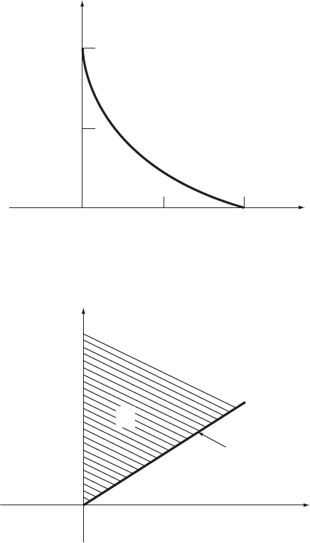
Finally, Equation (5.46) gives
This is shown graphically in Figure 5.17. It is an easy exercise to show that
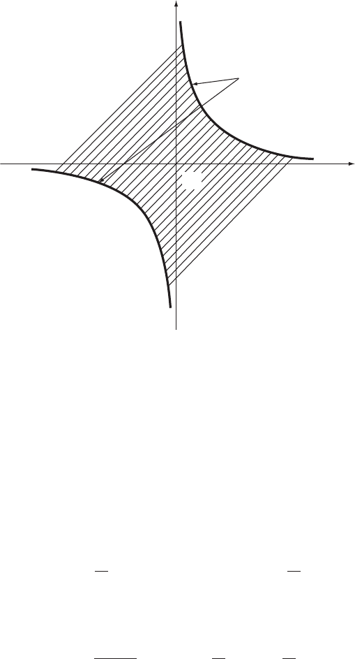
Ex ample 5. 12. Problem: let Y X
1
/X
2
where X
1
and X
2
are independent and
identically distributed according to
and similarly for X
2
. Determine f
Y
(y).
Answer: it follows from Equations (5.41) and (5.42) that
140
Fundamentals of Probability and Statistics for Engineers
f
X
1
x
1
2x
1
; for 0 x
1
1;
0; elsewhere;
f
X
2
x
2
2 x
2
2
; for 0 x
2
2;
0; elsewhere:
8
<
:
f
Y
y
Z
1
1
f
X
1
y
x
2
f
X
2
x
2
1
x
2
dx
2
;
Z
2
y
2
y
x
2
2 x
2
2
1
x
2
dx
2
; for 0 y 2;
0; elsewhere:
5:46
f
Y
y
2 yln y 1 ln 2; for 0 y 2;
0; elsewhere:
5:47
Z
2
0
f
Y
ydy1:
f
X
1
x
1
e
x
1
; for x
1
> 0;
0; elsewhere;
5:48
F
Y
y
Z
R
2
: x
1
=x
2
y
Z
f
X
1
X
2
x
1
; x
2
dx
1
dx
2
:
TLFeBOOK
The region R
2
for positive values of x
1
and x
2
is shown as the shaded area in
Figure 5.18. Hence,
y
f
Y
(
y
)
01
1
2
2
Figure 5. 17 Probability density function, f
Y
(y), in Example 5.11
x
1
x
2
—
=
y
R
2
x
2
x
1
Figure 5. 18 Region R
2
in Example 5.12
Functions of Random Variables
141
F
Y
y
Z
1
0
Z
x
2
y
0
f
X
1
X
2
x
1
; x
2
dx
1
dx
2
; for y > 0;
0; elsewhere:
8
<
:
TLFeBOOK

For independent X
1
and X
2
,
The pdf of Y is thus given by, on differentiating Equation (5.49) with respect
to y,
and, on substituting Equation (5.48) into Equation (5.50), it takes the form
Again, it is easy to check that
Example 5.13. To show that it is elementary to obtain solutions to problems
discussed in this section when X
1
,X
2
,..., and X
n
are discrete, consider again
Y X
1
/X
2
given that X
1
and X
2
are discrete and their joint probability mass
function (jpmf) p
X
1
X
2
(x
1
,x
2
) is tabulated in Table 5.1. In this case, the pmf of Y
is easily determined by assignment of probabilities p
X
1
X
2
(x
1
,x
2
) to the corres-
ponding values of y x
1
/x
2
. Thus, we obtain:
142
Fundamentals of Probability and Statistics for Engineers
F
Y
y
Z
1
0
Z
x
2
y
0
f
X
1
x
1
f
X
2
x
2
dx
1
dx
2
;
Z
1
0
F
X
1
x
2
yf
X
2
x
2
dx
2
; for y > 0;
0; elsewhere:
5:49
f
Y
y
Z
1
0
x
2
f
X
1
x
2
yf
X
2
x
2
dx
2
; for y > 0;
0; elsewhere;
8
>
<
>
:
5:50
f
Y
y
Z
1
0
x
2
e
x
2
y
e
x
2
dx
2
1
1 y
2
; for y > 0;
0; elsewhere:
8
>
<
>
:
5:51
Z
1
0
f
Y
ydy 1:
p
Y
y
0:5; for y
1
2
;
0:24 0:04 0:28; for y 1;
0:04; for y
3
2
;
0:06; for y 2;
0:12; for y 3:
8
>
>
>
>
>
>
>
>
<
>
>
>
>
>
>
>
>
:
TLFeBOOK

Example 5.14. Problem: in structural reliability studies, the probability of
failure q is defined by
where R and S represent, respectively, structural resistance and applied force.
Let R and S be independent random variables taking only positive values.
Determine q in terms of the probability distributions associated with R and S.
Answer: let Y R/S. Probability q can be expressed by
Identifying R and S with X
1
and X
2
, respectively, in Example 5.12, it follows
from Equation (5.49) that
Ex ample 5. 15. Problem: determine F
Y
(y) in terms of f
X
1
X
2
(x
1
,x
2
)when
1 2
).
Answer: now,
where region R
2
is shown in Figure 5.19. Thus
Table 5.1 Joint probability mass
function, p
X
1
X
2
(x
1
,x
2
), in Example 5.13
x
2
x
1
123
1 0.04 0.06 0.12
2 0.5 0.24 0.04
Functions of Random Variables
143
q PR S;
q P
R
S
1
PY 1F
Y
1:
q F
Y
1
Z
1
0
F
R
sf
S
sds:
F
Y
y
ZZ
R
2
: minx
1
;x
2
y
f
X
1
X
2
x
1
; x
2
dx
1
dx
2
;
F
Y
y
Z
y
1
Z
1
1
f
X
1
X
2
x
1
; x
2
dx
1
dx
2
Z
1
y
Z
y
1
f
X
1
X
2
x
1
; x
2
dx
1
dx
2
Z
y
1
Z
1
1
f
X
1
X
2
x
1
; x
2
dx
1
dx
2
Z
1
1
Z
y
1
f
X
1
X
2
x
1
; x
2
dx
1
dx
2
Z
y
1
Z
y
1
f
X
1
X
2
x
1
; x
2
dx
1
dx
2
F
X
2
yF
X
1
yF
X
1
X
2
y; y;
Y min(
X
,X
TLFeBOOK