Salcido A. (ed.) Cellular Automata - Simplicity Behind Complexity

Подождите немного. Документ загружается.

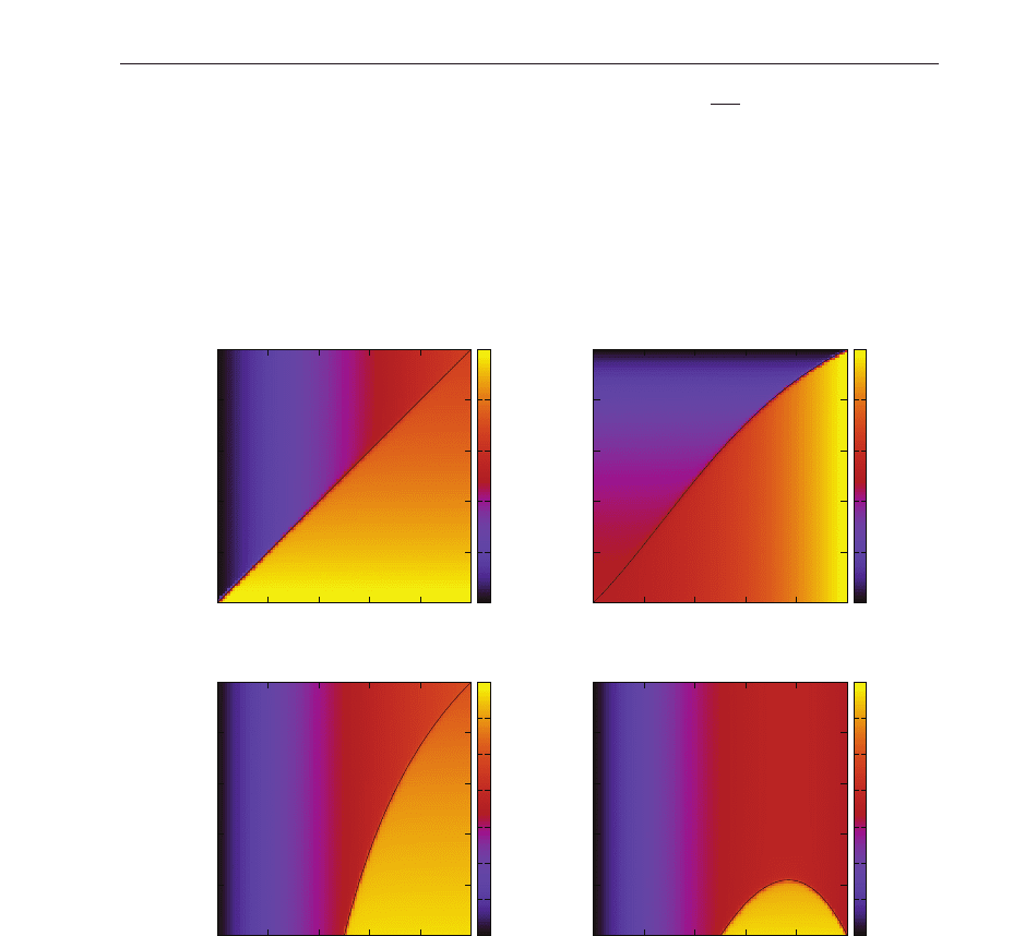
Rule 184

0 0.2 0.4 0.6 0.8 1

0.2

0.4

0.6

0.8

0.2

0.4

0.6

0.8

0 0.2 0.4 0.6 0.8 1

0.2

0.4

0.6

0.8

Fig. 3. Phase diagrams of rule 184 with the stochastic boundary condition (13). The average

density of 1s is illustrated. The phase transition line α

= β is also depicted.

We can adapt the boundary condition to the ECA with conserved density E

(xy)=(x −y)

t+1



− x

t+1

with probability α

t+1

with probability 1 − α

, x

t+1



− x

t+1

with probability 1 − β

t+1

with probability β

(14)

This is equivalent to the following evolution of probability distributions.

t+1

(x)=p

N+1

)

∑



,...,x



N+1

∏

i=1

δ(x

, f (x



i−1



i+1

))p



), (15)

where the conditional probabilities ρ

and ρ

are deﬁned as

(u|v)=αδ(E(uv),1)+(1 − α)δ (E(uv),0), p

(u|v)=(1 −β)δ(E(vu),1)+βδ(E(vu),0) .

(16)

As shown in Table 1, the rules with the conserved density are rules 14, 35, 43 and 142.

However, rule 43 is equivalent to rule 184 by block transformation 00, 11

→ 0 and 01, 10 → 1.

Namely, if we denote the transformation by b, the following equality holds:

(

) f

)

= f

184

(

b(x

)b(x

)

, (17)

where f

and f

184

are respective rule functions. Thus, rule 43 of size N + 2 with the stochastic

boundary condition (15) is transformed into rule 184 of size N

+ 1 with the stochastic

boundary condition (13) and accordingly exhibits the same nonequilibrium phase transition.

Similarly, rule 142 is transformed into rule 184 by another block transformation 01, 10

→ 0

and 00, 11

→ 1. In this case, the transformation is accompanied with change of parameter

values α

→ 1 − α, β → 1 − β. The phase transition of the same type occurs in this rule also.

Rules 14 and 35 are not equivalent to rule 184 and are considered in the next section. We only

mention here that the current function for rule 14 is J

(xyz)=−xy − (1 −x)(1 −y)z, and that

for rule 35 is J

(xyz)=x(1 − y)(1 −z).

For rules 56, we must have further consideration. The additive conserved quantity for this

rule has range 2. To make the conditional probability for boundary variables depend on

E, there must be more than two stochastic variables for each boundary. One way is using

more stochastic variables like p

−1

) and the other way is increasing the variables of

conditions like p

). In either way, there is another problem. The conserved density

407

Nonequilibrium Phase Transition of

Elementary Cellular Automata with a Single Conserved Quantity

can take three values 0, 1 and 2. If we want to study general cases, two parameters per

boundary are necessary. Thus, the boundary condition can be more complicated than Eqs.

(13) or (15). However, we can avoid these problems. Carefully looking at the time evolution

of rule 56, one can notice that block 111 does not appear in time t

≥ 1. In fact, no preimages

for block 111 exist for rule 56. This means that E

(xyz)=x + y + z −3xyz is equivalent to

(xyz)=x + y + z for t ≥ 1. Thus, rule 56 conserves the number of 1s for t ≥ 1. Such a

quantity was called an eventually conserved quantity in (Hattori and Takesue 1991). In the

case of stochastic boundary condition, block 111 can appear only at the ends of the system.

No 111 appears in the interior of the system. Therefore, we can use the boundary condition

(13) for rule 56. The rule function f

= x(1 − y)+(1 − x)yz satisﬁes the following equation,

(xyz) −y = x(1 −y) −y(1 −z ) −xyz. (18)

This is interpreted as that the current function for the eventually conserved quantity is J

(xy)=

x(1 − y).

Rule 11 has an eventually conserved quantity, too. In this case, block 101 has no preimages and

under the absence of 101, E

(xy)=(x −y)

becomes a conserved density. The corresponding

current function is J

(xyz)=x(1 − y)+(1 − x)yz. Therefore, the boundary condition (15) is

appropriate to this rule.

5. Application of the domain wall theory

The domain wall theory is applied to the ECA with the stochastic boundary condition as

follows. First we try to obtain the probability distribution of patterns of size three in the

stationary states. Let p

denote the probability distribution of block pattern starting from cell

i. For example, p

(000) means that the probability that x

i+1

i+2

= 000 and p

(0101) is the

probability that x

i+1

i+2

i+3

= 0101. In the stationary state, those probabilities satisfy the

following equations

∑



δ(x

, f (x



) f (x



) f (x



))p

i−1



). (19)

Assuming uniformity for p

and introducing decoupling approximation for the probability

distribution of larger size if necessary, we can obtain a set of stationary solutions which contain

the average density of the additive conserved quantity as a parameter. In particular, it is useful

to use the logic that if p

)=0, we must have p(x

)=0orp(x

)=0 to close

the equations consistently. Next, we try to adapt the solution to the left and right boundary

conditions. If the boundary condition (15) is employed, the following equations must hold at

the left boundary, namely

∑



δ(x

, f (x



) f (x



) f (x



))p



) (20)

and

)=p

). (21)

By solving the equations, the distribution in the left phase is determined and the average

density ρ

and current J

of the additive conserved quantity are obtained as functions of

parameter α. The right phase is determined in the similar manner and the average density ρ

and the average current J

is computed as functions of β. Once these quantities are obtained,

408

Cellular Automata - Simplicity Behind Complexity

we can apply the domain wall theory and the line of phase transition is calculated from the

condition J

= J

In (Takesue 2008) we showed how the above procedure works for rule 184. In that case, use

of the probability distributions of size two is sufﬁcient. In the following, we will discuss the

four rules 35, 14, 56 and 11 in this order.

5.1 Rule 35

If we assume uniformity, Eq. (19) becomes

(000)=p(1100)+p (111), p(001)=p (100)+p(1101),

(010)=p(101)+p (1001), p(011)=p (1000),

(100)=p(011)+p (0100), p(101)=p (0101),

(110)=p(0001), p(111)=p(0000). (22)

The sixth equation means p

(1101)=0, so we must have p(110)=0orp(101)=0. In the

former case, the ﬁrst and second equations mean that p

(000)=p(111) and p(001)=p(100).

Then, p

(0001)=p(1000)=0 is obtained from the eighth equation. Therefore, we have

(000)=p(011)=p (111)=0 and the remainings are determined as

(001)=p(100)=1 −ρ, p(010)=

, p

(101)=

−1, (23)

where ρ is the expectation value of E

(xy) and this solution makes sense only when

≤ ρ ≤ 1.

In the latter case, using approximation p

(0000)=

p(000)

p(00)

, we arrive at

(000)=

2 −3ρ

, p

(001)=

, p

(010)=

2 −ρ

(011)=

ρ(2 −3ρ)

2(2 − ρ)

(100)=

, p

(101)=0, p(110)=

ρ(2 −3ρ)

2(2 − ρ)

, p(111)=

(

2 −3ρ)

4(2 − ρ)

. (24)

This is the solution for 0

≤ ρ ≤

The connection condition (20) is written as

(000)=p

(1100)+p

(111), p

(001)=p

(100)+p

(1101),

(010)=p

(101)+p

(1001), p

(011)=p

(1000),

(100)=p

(011)+p

(0100), p

(101)=p

(0101),

(110)=p

(0001), p

(111)=p

(0000). (25)

As in Eq. (21), p

is written as p

(xyzw)=(αδ

x,1−y

+(1 −α)δ

(yzw). Then substitution of

the solution for 0

≤ ρ ≤

, (23), into p

satisﬁes the above equations if ρ = ρ

2α

2+α

. Notice

that as α varies from 0 to 1, ρ

varies from 0 to

. The stationary solution for ρ ≥

, (24),

cannot satisfy the above equations. At the right boundary p

N−2

N−1

) must satisfy

N−2

(000)=p

N−2

(1100)+p

N−2

(111), p

N−2

(001)=p

N−2

(100)+p

N−2

(1101),

N−2

(010)=p

N−2

(101)+p

N−3

(1001), p

N−2

(011)=p

N−3

(1000),

N−2

(100)=p

N−2

(011)+p

N−2

(0100), p

N−2

(101)=p

N−2

(0101),

N−2

(110)=p

N−3

(0001), p

N−2

(111)=p

N−3

(0000). (26)

409

Nonequilibrium Phase Transition of

Elementary Cellular Automata with a Single Conserved Quantity

Here the boundary condition is p

N−2

(xyzw)=[βδ

+(1 − β)δ

z,1−w

N−2

(xyz). In this case

substitution of (24) into p

N−2

satisﬁes the equations if ρ = ρ

2+β

. Because J(xyz)=

x(1 − y)(1 − z), the ﬂux in the left phase is J

= p

(100)=

2+α

and that in the right phase is

= p

N−2

(100)=

2+β

. Then, the velocity of the domain wall is obtained as

− J

−ρ

β − α

2 −α − αβ

(27)

Thus, if β

> α the left phase prevails, and if β < α the right phase does.

5.2 Rule 14

Equations for a uniform stationary state are

(000)=p(111)+p (0000)+p(11000), p(001)=p(0001)+p(1101)+p(11001),

(010)=p(101), p(011)=p(001),

(100)=p(011)+p (01000), p(101)=p(0101)+p( 01001),

(110)=p(001), p(111)=0. (28)

The ﬁrst and the eighth equations imply that p

(01000)=0. Thus, p(010)=0orp(100)=0

or p

(000)=0 must be satisﬁed to obtain a consistent solution. Case p(010)=0 leads to

(010)=p(101)=p (111)=0, p(001)=p(011)=p (100)=p(110)=

, p

(000)=1 −2ρ,

(29)

which is the solution for 0

≤ ρ ≤

. Case p(100)=0 leads to the solution p (101)=p(010)=

2ρ, p(000)=1 − 2ρ and the other entries are zeroes. In this case, block 000 and the other

two cannot coexist in a system, because if 000 coexists with some 1s, 001 and 100 should

have nonzero probability. Thus, this solution is not ergodic in the sense that time average

for a system does not agree with expectation with respect to this probability distribution.

Because we are interested in ergodic distribution only, we do not adopt this solution. In Case

(000)=0 we have the following solution

(000)=p(111)=0, p(001)=p(011)=p(100)=p(110)=

1 −ρ

, p

(010)=p(101)=ρ −

(30)

It corresponds to case

≤ ρ ≤ 1. The connection condition at the right end is given as

N−2

(000)=p

N−3

(111)+β[p

N−2

(000)+p

N−3

(1100)],

N−2

(001)=p

N−3

(1101)+(1 − β)[p

N−2

(000)+p

N−3

(1100)],

N−2

(010)=p

N−3

(101), p

N−2

(011)=p

N−2

(001),

N−2

(100)=p

N−3

(100)+βp

N−3

(0100),

N−2

(101)=p

N−3

(0101)+(1 − β)p

N−3

(0100),

N−2

(110)=p

N−3

(001), p

N−2

(111)=0. (31)

Substitution of the stationary solution for 0

≤ ρ ≤

, (29), into p

N−2

satisﬁes these equations

and the density of the conserved quantity is obtained as ρ

= ρ

2(1−β)

4−3β

. In addition, the

average current is given as

= −ρ

= −

2(1 − β)

4 −3β

. (32)

410

Cellular Automata - Simplicity Behind Complexity

The connection condition at the left end is given as

(000)=(1 − α)(p

(111)+p

(1000)) + p

(0000),

(001)=p

(0001)+(1 −α)( p

(101)+p

(1001)),

(010)=αp

(01), p

(011)=p

(001),

(100)=α(p

(11)+p

(1000)), p

(101)=α(p

(101)+p

(1001)),

(110)=(1 − α)p

(01), p

(111)=0. (33)

In this case, if either of the uniform stationary solutions is inserted into p

, the equations are

not satisﬁed. Instead, if we assume that p

equals the stationary solution for

≤ ρ ≤ 1, we

have

(000)=

(

1 −α)

4 −3α + α

, p

(001)=

1 −α

4 −3α + α

(010)=

4 −3α + α

, p

(011)=

1 −α

4 −3α + α

(100)=

α(1 −α)

4 −3α + α

, p

(101)=

4 −3α + α

(110)=

1 −α

4 −3α + α

, p

(111)=0. (34)

Note that only the property p

(000)=0 has been used to derive the above. The relation

between α and ρ should be obtained by p

(000)+p

(100)=p

(000)+p

(001)=

1−ρ

, which

leads to

= ρ

2 −α + α

4 −3α + α

. (35)

However, this is inconsistent with another condition p

(001)+p

(101)=p

(010)+

(011)=

. Namely, the two conditions cannot be satisﬁed at the same time by the uniform

solution. This inconsistency is resolved by considering a periodic solution for the stationary

distribution. If we assume period two for the distribution and denote the distribution function

starting from an even-numbered cell by p

and that starting from an odd-numbered cell by

, Eqs. 28 are replaced with

(000)=p

(111)+p

(0000)+p

(10000), p

(001)=p

(0001)+p

(1101)+p

(11001),

(010)=p

(101), p

(011)=p

(001),

(100)=p

(011)+p

(01000), p

(101)=p

(0101)+p

(01001),

(110)=p

(001) p

(111)=0 (36)

and those with p

and p

interchanged. For ρ ≥

, we have the solution similar to (30) except

(010)=p

(101)=ρ −

+ , p

(101)=p

(010)=ρ −

−, (37)

where  is a parameter satisfying

−(ρ −1/2) ≤  ≤ ρ −1/2. Then, if we assume p

= p

with



= −

α(1 −α)

2(4 − 3α + α

)

, (38)

411

Nonequilibrium Phase Transition of

Elementary Cellular Automata with a Single Conserved Quantity

the solution is consistently connected to Eq. 34. Thus, the average density (35) is still correct

and the average current in the left phase is given by

= −p

(001) − p

(110) − p

(111)=−

2(1 − α)

4 −3α + α

(39)

The phase transition line is calculated via J

= J

and the result is

α(1 + α)

1 + α

. (40)

5.3 Rule 56

Equations for a uniform stationary state are

(000)=p(0000)+p (1111)+p(00010), p(001)=p(0010)+p(1110)+p( 00011),

(010)=p(0011)+p (100)+p(1010), p(011)=p(1011),

(100)=p(1000)+p (0111)+p(10010), p(101)=p(0110)+p(1010)+p( 10011),

(110)=p(1011), p(111)=0. (41)

The ﬁrst and the eighth equations leads to p

(00011)=0 and the second equation means

(10011)=0. Thus p(0011)=0 must hold. This implies that p(001 )=0orp (011)=0. In the

former case, we have p

(001)=p(100)=p(111)=0. Then, for the state to be ergodic p(000)

must vanish and the remainings are determined as

(010)=2 −3ρ, p(011)=p(110)=2ρ −1, p(101)=1 −ρ, (42)

where ρ is the density of 1s. This solution makes sense when

≤ ρ ≤

. Note that p(111)=0

means the maximum value of ρ is

. In the latter case, p(011)=p(110)=p(111)=0 and the

others are

(000)=1 −2ρ − a, p(001)=p(100)=a, p(010)=ρ, p(101)=ρ − a, (43)

where a is a real number in the region 0

≤ a ≤ min(ρ,1−2ρ). This is the solution for 0 ≤ ρ ≤

. The connection at the left end is given by

(000)=(1 −α)[p

(000)+p

(0010)],

(001)=(1 −α)[p

(010)+p

(0011)] + αp

(110),

(010)=(1 − α)p

(011)+p

(100)+p

(1010), p

(011)=p

(1011),

(100)=α[p

(000)+p

(0010)],

(101)=α[p

(010)+p

(0011)]+(1 − α)p

(110),

(110)=αp

(011), p

(111)=0. (44)

This is satisﬁed by the bulk solution for 0

≤ ρ ≤

with ρ = ρ

1+α

and a =

α(1−α)

1+α

. The

average current in this phase is

= p

(100)+p

(101)=ρ

1 + α

. (45)

412

Cellular Automata - Simplicity Behind Complexity

The connection at the right end is given as

N−2

(000)=p

N−3

(0000)+βp

N−3

(0001),

N−2

(001)=p

N−3

(0010)+(1 − β)p

N−3

(0001),

N−2

(010)=p

N−2

(100)+p

N−3

(0011)+βp

N−2

(101), p

N−2

(011)=p

N−2

(1011),

N−2

(100)=p

N−3

(1000)+βp

N−3

(1001),

N−2

(101)=p

N−3

(0110)+p

N−3

(1010)+(1 − β)p

N−3

(1001),

N−2

(110)=p

N−3

(1011), p

N−2

(111)=0. (46)

This is satisﬁed by substitution of the stationary solution with ρ

= ρ

2−β

3−β

into p

N−2

. The

average current is given as

= p

N−2

(100)+p

N−2

(101)=1 − ρ

3 − β

(47)

The phase transition occurs when J

= J

, which is given by

= 2 −

. (48)

5.4 Rule 11

Let us assume period-two stationary solutions from the beginning. The equations are

(000)=p

(111)+p

(1010)+p

(10100), p

(001)=p

(100)+p

(1011),

(010)=p

(1011)+p

(10010), p

(011)=p

(1000)+p

(10011),

(100)=p

(011)+p

(0010), p

(101)=0,

(110)=p

(0011)+p

(00010) p

(111)=p

(0000)+p

(00010). (49)

and those with p

and p

interchanged. The sixth equation implies the second and third

terms in the rhs of the ﬁrst equation vanish. Thus we obtain p

(000)=p

(111). In the same

manner, p

(111)=p

(000), p

(001)=p

(100) and p

(001)=p

(100) are obtained. The

eighth equation is rewritten as p

(111)=p

(000) − p

(00010) and substitution of p

(111)=

(000) leads to p

(00010)=0. Thus at least one of p

(000), p

(001),orp

(010) must vanish.

Similarly, one of p

(000), p

(001),orp

(010) must vanish. However, if p

(001)=0, p

(010)

must vanish, because p

(01)=p

(101)+p

(001)=0. Thus, the case p

(001)=0 is included

in the case p

(010)=0. Moreover, if p

(010)=0, p

(10010)=0 and accordingly p

(0010)=

(010)=0. Thus, it is sufﬁcient to investigate the two cases p

(000)=p

(000)=0 and

(010)=p

(010)=0. The former case leads to the following uniform (namely p

= p

= p)

solution

(000)=p(101)=p (111)=0, p(001)=p(100)=

(010)=2ρ −1, p(011)=p(110)=1 −

ρ, (50)

413

Nonequilibrium Phase Transition of

Elementary Cellular Automata with a Single Conserved Quantity

where the average density ρ of eventually conserved quantity satisﬁes

≤ ρ ≤

. In the latter

case, we have the period-two solution as

(000)=

−ρ + , p

(000)=

−ρ − ,

(001)=p

(100)=

−, p

(001)=p

(100)=

+ ,

(010)=p

(101)=0, p

(010)=p

(101)=0,

(011)=p

(110)=

+ , p

(011)=p

(110)=

−,

(111)=

−ρ − , p

(111)=

−ρ + , (51)

where 0

≤ ρ ≤

and 0 ≤  ≤ min(ρ/2,1/2 −ρ ). Connection at the left end is given by

(000)=(1 − α)p

(11)+p

(1010)+αp

(0100), p

(001)=p

(100),

(010)=α[p

(011)+p

(0010)], p

(011)=α[p

(000)+p

(0011)],

(100)=αp

(11)+(1 −α)p

(010), p

(101)=0,

(110)=(1 − α)[p

(011)+p

(0010)], p

(111)=(1 −α)[p

(000)+p

(0011)].

(52)

These equations can be solved with the assumption that p

is given by p

in Eq. (51). As the

result, p

is obtained as

(000)=K



1 −α − α

+ 2α



, p

(001)=Kα



1 + α −2α



(010)=Kα

, p

(011)=Kα,

(100)=Kα



1 + α −2α



, p

(101)=0,

(110)=Kα(1 −α), p

(111)=K(1 −α), (53)

where K

=(2 + 2α + α

− 2α

)

−1

. The relations among ρ

,  and α are obtained via the

consistency between p

and p

= 1 −2K =

α(2 + α −2α

)

2 + 2α + α

−2α

,  =

(1 − α)

2 + 2α + α

−2α

. (54)

The conserved current in the left domain is J

= p

(011)+p

(100)=ρ

= Kα( 2 + α − 2α

Connection at the right end is given by the condition

N−2

(000)=p

N−3

(000)+βp

N−3

(0001), p

N−2

(001)=p

N−2

(100)

N−2

(010)=(1 − β)p

N−3

(1001), p

N−2

(011)=p

N−3

(1000)+βp

N−3

(1001),

N−2

(100)=p

N−3

(011)+p

N−3

(0010), p

N−2

(101)=0

N−2

(110)=p

N−3

(0011)+(1 − β)p

N−3

(0001), p

N−2

(111)=p

N−3

(0000)+βp

N−3

(0001).

(55)

These equations are satisﬁed by the substitution of (50) into p

N−2

. Relation between ρ

and β

is given by

3 + β

. (56)

414

Cellular Automata - Simplicity Behind Complexity

And the average current in the right phase is given as J

= 1 −ρ

1+β

3+β

. The phase transition

occurs when J

= J

, that is

=(2α − 1)(1 −α

). (57)

5.5 Numerical simulations

We carried out simulations of the four rules for various α and β. The result is illustrated in

Fig. 4. As is seen from the ﬁgure, the agreement of the theoretically obtained phase transition

line and numerical results is excellent. Values of the density and the current also show a nice

agreement between the theory and numerical results.

Rule 35

0 0.2 0.4 0.6 0.8 1

0.2

0.4

0.6

0.8

0.2

0.4

0.6

0.8

0 0.2 0.4 0.6 0.8 1

0.2

0.4

0.6

0.8

Rule 14

0 0.2 0.4 0.6 0.8 1

0.2

0.4

0.6

0.8

0.2

0.4

0.6

0.8

0 0.2 0.4 0.6 0.8 1

0.2

0.4

0.6

0.8

Rule 56

0 0.2 0.4 0.6 0.8 1

0.2

0.4

0.6

0.8

0.1

0.2

0.3

0.4

0.5

0.6

0.7

0 0.2 0.4 0.6 0.8 1

0.2

0.4

0.6

0.8

Rule 11

0 0.2 0.4 0.6 0.8 1

0.2

0.4

0.6

0.8

0.1

0.2

0.3

0.4

0.5

0.6

0.7

0 0.2 0.4 0.6 0.8 1

0.2

0.4

0.6

0.8

Fig. 4. Phase diagrams of the ECAs. The density of the conserved quantity for each rule and

the theoretically obtained phase transition lines are illustrated.

6. Diffusion of the domain wall

The velocity of the domain wall V vanishes on the phase transition line. It does not mean that

the domain wall stops somewhere but implies diffusive motion. Eq. (11) can be interpreted

as that the domain wall undergoes a random walk with the rate of hopping to the right is

415

Nonequilibrium Phase Transition of

Elementary Cellular Automata with a Single Conserved Quantity

/(ρ

−ρ

) and that to the left is J

/(ρ

−ρ

). Then the diffusion constant is given by

+ J

2(ρ

−ρ

)

. (58)

On the phase transition line, the drift velocity vanishes and pure diffusive motion appears.

This diffusive motion leads to interesting power-law in the power spectral density for the time

sequence of the conserved density at a position (Takesue et al 2003). This is ﬁrst observed for

the TASEP and our ECA rules share this phenomenon. Now we consider the case where the

conserved density is E

(xy)=(x − y)

. The case of E(x )=x is simpler than that. The power

spectral density is deﬁned as follows. Record a time sequence of E

) for a ﬁxed i and

≤ t < T. Fourier components of the time sequence are calculated as

T−1

∑

t=0



) − ρ



−iω

, (59)

where ω

2πn

(n = 0, 1, 2, . . . , T) and ρ

is the expectation value of E(x

i+1

) in the

stationary state. Then, the power spectral density is deﬁned as

(ω

)=T

, (60)

where

denotes the sample average. Now, we approximate the motion of the domain wall

by Brownian motion. In this approximation, the density proﬁle is represented as

(x, t)=ρ

+(ρ

−ρ

)θ(x −X(t)), (61)

where ρ

(x, t) is the coarse-grained density proﬁle at time t and position x, X(t) is a

Brownian motion with diffusion constant D, θ

(x) is the Heaviside function. Applying the

Wiener-Khinchin theorem, we obtain the power spectral density as

(ω)=

√

(

−ρ

)

−3/2

. (62)

The power spectral density for rule 35 is shown in Fig. 5. The power law behavior is seen in

a region of ω. The agreement with the theory is very good including the prefactor. Also in

the other rules, the power spectral density exhibits the power law on the phase transition line.

The prefactor agrees with the theoretical value in every case except in rule 11, where a small

deviation is seen. The deviation is expected to decrease as the system size increases.

7. Discussion and conclusion

We have seen that the ECA with a single additive conserved quantity show a nonequilibrium

phase transition of the same type as in the ASEP. The phase transition line is precisely

determined by applying the domain wall theory. In these rules, there occurs only the

ﬁrst-order phase transition and no maximal current phase is observed. It is to be investigated

why the maximal current phase does not exist in the ECA and in what kind of CA it appear.

The connection between the stationary distribution and the boundary condition depends on

the conditional probability. We discuss some possible generalizations. For example, we can

consider the following conditional probability.

(1|0)=α, p

(0|0)=1 −α, p

(0|1)=γ, p

(1|1)=1 −γ, (63)

416

Cellular Automata - Simplicity Behind Complexity