Nair S. Advanced Topics in Applied Mathematics: For Engineering and the Physical Sciences

Подождите немного. Документ загружается.

Integral Equations 69

We notice that k

(1)

, k

(3)

, k

(5)

, etc., contain sin(x +ξ)and k

(2)

, k

(4)

, k

(6)

etc., contain cos(x −ξ). The Neumann series can be written as

g(x, ξ)=



1 +

+···





sin(x +ξ)+

λπ

cos(x −ξ)



(2.83)

When |λ|< 2/π , we may sum the series to ﬁnd

g(x, ξ)=

1 −λ

[sin(x +ξ)+

λπ

cos(x −ξ)]. (2.84)

The following example shows, in fact, this expression is valid even

when |λ|> 2/π .

2.7.2 Example: Direct Calculation of the Resolvent Kernel

From the equation

u(x) =λ



[sinxcosξ +cosx sinξ ]u(ξ) dξ +f (x), (2.85)

by deﬁning

=f ,cos, c

=f ,sin, (2.86)

we have

u(x) =λ[c

sinx +c

cosx]+f (x). (2.87)

Multiplying this by cosx and integrating, we ﬁnd

λπ

+f ,cos. (2.88)

Similarly, using sinx,

λπ

+f ,sin. (2.89)

Solving for c

and c

1 −λ

[f ,cos+

λπ

f ,sin], (2.90)

70 Advanced Topics in Applied Mathematics

1 −λ

[f ,sin+

λπ

f ,cos]. (2.91)

Substituting these in the expression (2.87),

u(x) =f (x) +

1 −λ



[sin(x +ξ)+

λπ

cos(x −ξ)]f (ξ )dξ .

(2.92)

The resolvent kernel can be seen as

g(x, ξ)=

1 −λ

[sin(x +ξ)+

λπ

cos(x −ξ)], (2.93)

which is valid for all values of λ, except when λ is an eigenvalue, (i.e.,

λ =±2/π).

2.8 QUADRATIC FORMS

Associated with a symmetric kernel k(x, ξ), we have the quadratic form

J[u]=



k(x,ξ)u(x)u(ξ)dξ dx. (2.94)

If the functions u are selected from the set satisfying u=1, the

extremum values of J can be found by setting the ﬁrst variation of the

modiﬁed functional

∗

[u]=J[u]−µ





dx −1



(2.95)

to zero. Here, µ is a Lagrange multiplier. Using the calculus of

variations, we obtain the eigenvalue problem

u(x) =λ



k(x,ξ)u(ξ)dξ , (2.96)

where λ = 1/µ. For a particular normalized eigenfunction u

, Eq.

(2.96) becomes

(x) =λ



k(x,ξ)u

(ξ)dξ . (2.97)

Integral Equations 71

Multiplying both sides of Eq. (2.97)byu

(x) and integrating, we ﬁnd

1 =λ

J[u

]. (2.98)

This shows that the extremum values of J corresponding to the

eigenfunctions satisfy

J[u

. (2.99)

2.9 EXPANSION THEOREMS FOR

SYMMETRIC KERNELS

We state two expansion theorems without proof:

I. If k(x,ξ) is degenerate or if it has a ﬁnite number of eigenvalues

of one sign (e.g., an inﬁnite number of positive eigenvalues and a

ﬁnite number of negative ones), it has the expansion

k(x,ξ)=



(x)u

(ξ)

, (2.100)

where N →∞when there are inﬁnite eigenvalues.

This is known as Mercer’s theorem.

II. For general symmetric kernels that are uniformly continuous in

their variables x and ξ , the relation

f (x) =



k(x,ξ)g(ξ )dξ , (2.101)

where g is a piecewise continuous function, can be considered

as an integral transformation of g with respect to the kernel k.

Functions f obtained in this way can be expanded in terms of the

eigenfunctions of k in the form

f (x) =

∞



(x). (2.102)

72 Advanced Topics in Applied Mathematics

For the proofs of Eqs. (2.100) and (2.102), the reader may consult

CourantandHilbert(1953).Thesecondexpansiontheoremshows

that the iterated kernel k

(2)

(x,ξ) has the form

(2)

(x,ξ)=

∞



(x). (2.103)

2.10 EIGENFUNCTIONS BY ITERATION

Solutions of the eigenvalue problem

u(x) =λ



k(x,ξ)u(ξ)dξ (2.104)

may be approximated by iterative means as follows: We choose a nor-

malized function u

(0)

and use it on the right-hand side of Eq. (2.104).

We, again, normalize the result of the integration and call it u

(1)

to use

in subsequent iterations. This procedure creates a sequence of func-

tions that would converge to an eigenfunction u

corresponding to the

eigenvalue with smallest value of |λ|.

To see the validity of this procedure, we observe the following: By

the second expansion theorem, u

(1)

will have the form

(1)

∞



(x). (2.105)

The next iteration gives

(2)

∞



(x)

(2.106)

and

(n)

∞



(x)

(n−1)

. (2.107)

If λ

is the smallest eigenvalue magnitude, we can write

(n)

n−1







n−1

+···



. (2.108)

Integral Equations 73

As n →∞, all the terms except the u

term go to zero. The normaliza-

tions will get rid off the constants multiplying u

. Once u

is known, λ

can be obtained from



k(x,ξ)u(ξ) dξ =

(x)

. (2.109)

This iterative method is known as Kellogg’s method.

To use this approach for higher eigenfunctions, we must make sure

our starting function is orthogonal to u

, and after each iteration the

orthogonality has to be reimposed. If the kernel satisﬁes the condi-

tions for the expansion theorem of Eq. (2.100), we may work with the

alternate kernel,

k = k(x, ξ)−

(x)u

(ξ)

, (2.110)

to ﬁnd the second eigenfunction.

2.11 BOUND RELATIONS

Let us assume the eigenvalue λ

has M eigenfunctions u

(m =1,2,..., M). Using the Bessel inequality with the norm of k(x,ξ)

with ξ and its projections on the M orthonormal eigenfunctions, we

have



(x,ξ)dξ ≥



m=1





k(x,ξ)u

(ξ) dξ





m=1

(x)

. (2.111)

Integrating with x,weget

M ≤λ



(x,ξ)dξdx. (2.112)

This puts an upper bound on the number of degenerate eigenfunctions.

If we use all eigenfunctions (discarding the double index notation

for degenerate ones), we have



(x,ξ)dξ ≥



i=1





k(x,ξ)u

(ξ) dξ





i=1

(x)

. (2.113)

74 Advanced Topics in Applied Mathematics

Again, integrating with x,weﬁnd



i=1

≤



(x,ξ)dξdx. (2.114)

2.12 APPROXIMATE SOLUTION

There are a number of ways of ﬁnding approximate solutions of inte-

gral equations. These range from semianalytic to purely numerical

approaches.

2.12.1 Approximate Kernel

We may replace the given kernel by an approximate kernel using N

orthonormal functions v

k(x,ξ)=



(x)v

(ξ), (2.115)

where the coefﬁcient functions are found from

(x) =k(x, ξ),v

(ξ). (2.116)

Now we have an approximate degenerate kernel.

2.12.2 Approximate Solution

To solve

u(x) =



k(x,ξ)u(ξ) dξ +f (x), (2.117)

we assume a functional expansion for the unknown u in the form

u(x) =



i=1

(x), (2.118)

Integral Equations 75

where v

(x) are from a chosen orthonormal sequence. The integral

equation reduces to



i=1

(x) =f (x), φ

(x) ≡v

(x) −



k(x,ξ)v

(ξ) dξ. (2.119)

A general way to solve for the unknown constants a

is given by the

Petrov-Galerkin method. If f (x) happens to be a linear combination of

the known functions φ

, we have a unique solution for the unknowns

. Otherwise, the error

e(x) ≡



−f (2.120)

will not be zero almost everywhere. In the Petrov-Galerkin method,

we choose a sequence of N independent functions ψ

and let the

projections of the error on these functions vanish. That is,



φ

,ψ

=f ,ψ

, j = 1,2, ...,N. (2.121)

For a symmetric kernel, we may choose ψ

to obtain a symmetric

matrix problem.

2.12.3 Numerical Solution

We begin by discretizing the interval [a,b] into N points, ξ

, i =

1,2, ...,N. Let u

= u(ξ

). The integral with k can be approximated

by the trapezoidal or the Simpson’s rule for numerical integration, for

example



k(x,ξ)u(ξ) dξ =



k(x,ξ

, (2.122)

where w

are the weight coefﬁcients of the particular numerical

integration scheme. For example, the trapezoidal rule has

, w

=1, , ..., (2.123)

76 Advanced Topics in Applied Mathematics

and Simpson’s rule has

, w

, .... (2.124)

Then

u(x) =



k(x,ξ

+f (x). (2.125)

We may use the method of collocation in which the error is made

exactly zero at N points. In our case, we choose these points as x

With

=k(x

,ξ

, b

=f (x

), (2.126)

we get

[I −A]u = b, (2.127)

where u and b are N vectors.

In all the three preceding approximation methods, integrals may

be evaluated numerically if necessary.

2.13 VOLTERRA EQUATION

Introducing a parameter λ, the Volterra equation given in Eq. (2.8)

can be written as

u(x) =λ



k(x,ξ)u(ξ) dξ +f (x). (2.128)

For continuity, the kernel has to satisfy k(x,x) = 0.

Using iterated kernels

(n)

(x,ξ)=



(n−1)

(x,η)k(η,ξ)dη, k

(1)

(x,ξ)= k(x,ξ), (2.129)

the Neumann series for this Volterra equation is obtained as

u(x) =f (x) +

∞



n=1



(n)

(x,ξ)f (ξ) dξ. (2.130)

Integral Equations 77

If we stipulate that k and f are bounded functions, with

|k|< M, |f | < F , (2.131)

we get





k(x,ξ)f (ξ) dξ



< MF(x −a)

and





(n)

(x,ξ)f (ξ) dξ



< M

(x −a)

. (2.132)

As n →∞, the Neumann series for u uniformly converges, and we

have a unique solution for the Volterra equation.

In special cases, by differentiating both sides, a Volterra equation

may be converted to a differential equation.

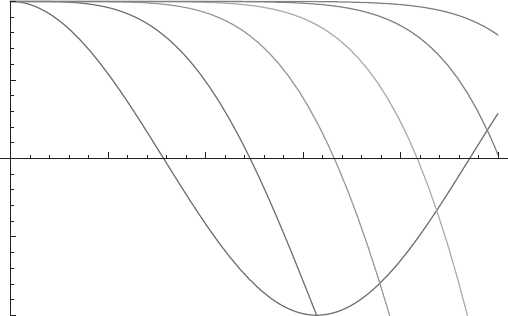
2.13.1 Example: Volterra Equation

The equation

u(x) =



sin(x −ξ)u(ξ )dξ +cos(x) (2.133)

has a slowly converging iterative solution. The ﬁrst ﬁve iterative

solutions are shown below.

(0)

=cosx,

(1)

=cosx +

sinx,

(2)

=cosx −

{xcosx −5sin x}

(3)

=cosx −



xcosx +



−33 +x



sinx



(4)

=cosx +

384





−87 +x



cosx +



279 −14x



sinx



(5)

=cosx +

3840





−195 +4x



cosx +



2895 −185x



sinx



Noting that the kernel has the cyclic property that it returns to its

initial form after two differentiations, by differentiating the integral

78 Advanced Topics in Applied Mathematics

1 2 3 4 5

–0.5

–1.0

0.5

1.0

Figure 2.1. Plots of the functions u

(0)

to u

(5)

with higher iterates getting closer to the

exact solution u = 1.

equation, we ﬁnd





cos(x −ξ)u(ξ )dξ −sinx, (2.134)



=0, (2.135)

where we have used Eq. (2.133) to eliminate the integral of the

unknown function u. We need two boundary conditions to go with this

second-order equation. From Eq. (2.133), we get u(0) = 1. From the

derivative of u, we ﬁnd u



(0) =0. The unique solution of the differential

equation is

u(x) =1. (2.136)

2.14 EQUATIONS OF THE FIRST KIND

We may investigate equations of the ﬁrst kind,



k(x,ξ)u(ξ) dξ = f (x), (2.137)

usingthesecondexpansiontheoremstatedinSection2.9.Thistheorem

states that if k is continuous and symmetric, f has an expansion in terms