Nair S. Advanced Topics in Applied Mathematics: For Engineering and the Physical Sciences
Подождите немного. Документ загружается.

Fourier Transforms 129
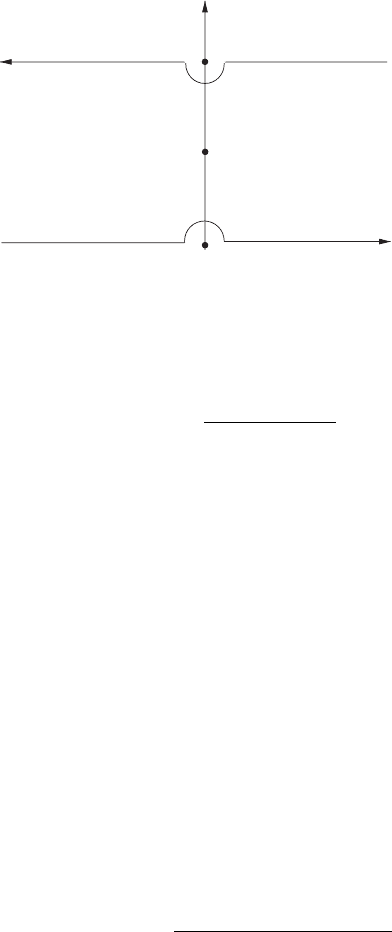
ξ
η
C
C
1
π
2π
0
Figure 3.9. Contour in the complex ζ plane.
On C
1
, ζ = ξ +2πi and
C
1
f (ζ )dζ =
−∞
∞
e
2π(ic+x)+(c−ix)ξ
sinh(ξ +2πi
dξ
=−e
2π(ic+x)
∞
−∞
f (ξ )dξ
=−e
2π(ic+x)
I. (3.169)
The residues are
Res(0) =1,
Res(πi) =−e
π(ic+x)
,
Res(2πi) =e
2π(ic+x)
.
As the points ζ =0andζ =2π i are on the contour, the Cauchy principal
values of the integrals through them give half the residues. Thus,
(1 −e
2π(ic+x)
)I = πi(1 +e
2π(ic+x)
−2e
π(ic+x)
),
I = πi
(1 −e
π(ic+x)
)
2
(1 −e
π(ic+x)
)(1 +e
π(ic+x)
)

130 Advanced Topics in Applied Mathematics
=πi
1 −e
π(ic+x)
1 +e
π(ic+x)
1 +e
π(−ic+x)
1 +e
π(−ic+x)
=π
sinπc −i sinhπx
cosπ c +coshπ c
. (3.170)
Using this in Eqs. (3.165) and (3.166),
g
0
(x,y) =
π
2a
2
sinπ ¯y/a
coshπx/a +cosπ ¯y/a
, (3.171)
g
1
(x,y) =
π
2a
2
sinπy/a
coshπx/a +cosπ y/a
, (3.172)
where ¯y =a −y.
3. Transient Heat Conduction in a Semi-infinite Rod
Consider a semi-infinite rod occupying 0 < x < ∞. The transient
relative temperature u(x,t) satisfies
κ
∂
2
u
∂x
2
=
∂u
∂t
, (3.173)
where κ is the diffusivity. The boundary conditions are
u(0,t) = 0, u →0asx →∞. (3.174)
The initial temperature distribution is given as
u(x,0) =f (x), (3.175)
with f (0) = 0andf → 0asx →∞. For a semi-infinite domain with
u(0,t) prescribed, we use the Fourier Sine transform.
U(ξ, t) =F
s
[u(x,t)], F
s
(ξ) =F
s
[f (x)], (3.176)
F
s
∂
2
u
∂x
2
=−ξ
2
U. (3.177)
Taking the transform of Eq. (3.173), we have
dU
dt
+κξ
2
U = 0, (3.178)
Fourier Transforms 131
which has the solution
U(ξ, t) =Ae
−κtξ
2
, (3.179)
where A is found from the initial condition, U(ξ ,0) =A =F
s
(ξ). Thus,
U(ξ, t) =F
s
(ξ)e
−κtξ
2
. (3.180)
For special initial temperature distributions, such as
f (x) =u
0
xe
−x
2
/(4a
2
)
, (3.181)
we have from Eq. (3.84)
F(ξ ) = u
0
(2
√
a)
3
ξe
−a
2
ξ
2
, (3.182)
U(ξ, t) =u
0
(2
√
a)
3
ξe
−(a
2
+κt)ξ
2
. (3.183)
Inverting this gives
u(x,t) =
u
0
x
(1 +κt/a
2
)
3/2
e
−x
2
/[4(a
2
+κt)]
. (3.184)
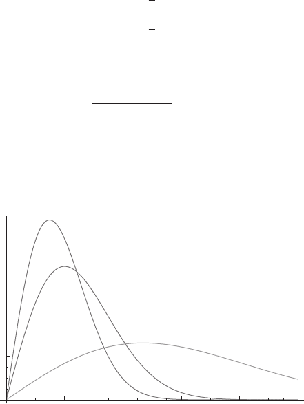
Figure 3.10 shows the peak temperature diminishing and moving
to the right as time passes.
2 4 6 8 10
0.2
0.4
0.6
0.8
Figure 3.10. Temperature distributions u/u
0
for t =0.1,1.0,10.0 when a
2
=κ =1.

132 Advanced Topics in Applied Mathematics
In a more general scenario, we would like to keep f (x) arbitrary and
to obtain the Green’s function to write the solution in a convolutional
form. To this end, from Eq. (3.123), we have
F
−1
s
[F
s
G
c
]=
1
√
2π
∞
0
f (t)[g(|x −t|−g(x +t)]dt, (3.185)
where
G
c
=e
−κtξ
2
, g(x) =
1
√
2κt
e
−x
2
/(4κt)
. (3.186)
Thus,
u(x,t) =
1
√
4πκt
∞
0
f (x
)[e
−(x−x
)
2
/(4κt)
−e
−(x+x
)
2
/(4κt)
]dx
. (3.187)
4. Transient Heat Conduction in a Rod with Radiation Condition
Here we reconsider the previous heat conduction problem with the
boundary condition at x = 0 changed to the radiation condition
(Newton’s law of cooling):
∂u
∂x
(0,t) −hu(0, t) =0. (3.188)
Using the mixed trigonometric transform,
U
R
(ξ, t) =F
R
[u(x,t)]=
2
π
∞
0
u(x,t)[ξ cosξx +hsin ξx]dx, (3.189)
we obtain
∂U
R
∂t
=−κξ
2
U
R
. (3.190)
The solution of this equation satisfying the initial condition, U
R
(ξ,0) =
F
R
(ξ),is
U
R
(ξ, t) =F
R
(ξ)e
−κtξ
2
. (3.191)
Using the relation (3.131) between the mixed transform and the
Sine transform,
U
R
=−F
s
∂u
∂x
−hu
, F
R
=−F
s
[g], (3.192)

Fourier Transforms 133
where
g ≡
∂f
∂x
−hf . (3.193)
Then
∂u
∂x
−hu =F
−1
s
2
π
e
−κtξ
2
∞
0
g(x
) sin ξx
dx
=
2
π
∞
0
∞
0
g(x
)e
−κtξ
2
sinξxsin ξ x
dx
dξ
=
1
π
∞
0
∞
0
g(x
)e
−κtξ
2
[cos(x −x
)ξ −cos(x +x
)ξ]dξ dx
=
1
√
4πκt
∞
0
g(x
)[e
−(x−x
)
2
/(4κt)
−e
−(x+x
)
2
/(4κt)
]dx
,
u =
1
√
4πκt
∞
0
g(x
)
∂
∂x
−h
−1
[e
−(x−x
)
2
/(4κt)
−e
−(x+x
)
2
/(4κt)
]dx
.
(3.194)
Next, we want to obtain the result of the inverse differential operator
acting on the x-dependent Gaussian functions inside the integral. This
is equivalent to seeking a solution of the differential equation
∂v
∂x
−hv = e
−(x−x
)
2
/(4κt)
−e
−(x+x
)
2
/(4κt)
. (3.195)
Note that v(x) satisfies the radiation boundary condition at x = 0. We
may solve for v using superposition by considering only the first term
on the right-hand side. Using an integrating factor,
∂(e
−hx
v)
∂x
=exp
−
x
2
−2xa +4κhtx +a
2
4κt
, (3.196)
where a =±x
. Completing the square,
∂(e
−hx
v)
∂x
=exp
(a −2κht)
2
−a
2
4κt
exp
−
(x −a +2κht)
2
4κt
=exp(−ha +κh
2
t) exp
−
(x −a +2κht)
2
4κt
. (3.197)

134 Advanced Topics in Applied Mathematics
Integrating both sides, we obtain
v =
√
πκt exp[h(x −a +κht)]erf
x −a +2κht
√
4κt
. (3.198)
With this, superimposing the two expressions for v corresponding to
a =±x
, the solution given in Eq. (3.194) can be written as
u =
1
2
∞
0
g(x
)[w(x −x
) −w(x +x
)]dx
, (3.199)
where
w(x) =e
h(x+κht)
erf
x +2κht
√
4κt
. (3.200)
5. Transient Heat Conduction in an Infinite Plate
The diffusion equation and the initial condition for the relative
temperature u are
κ∇
2
u(x,y,t) =
∂u
∂t
, u(x,y,0) = f (x, y), (3.201)
where f and u go to zero as
x
2
+y
2
→∞.
Using the double Fourier transform,
F [u(x, y,t), x → ξ, y → η]=U(ξ ,η,t), (3.202)
F [f (x, y),x →ξ,y →η]=F(ξ ,η), (3.203)
the differential equation can be written as
dU
dt
=−κ(ξ
2
+η
2
)U, (3.204)
which has the solution satisfying the given initial condition,
u =F(ξ ,η)e
−κt(ξ
2
+η
2
)
. (3.205)
The inverse transform of the exponential term can be found by con-
sidering it as a product of a function of ξ and a function of η.
g(x, y,t) =F
−1
[e
−κt(ξ
2
+η
2
)
]=
1
2κt
e
−(x
2
+y
2
)/(4κt)
. (3.206)

Fourier Transforms 135
Using the convolution theorem, the solution can be written as
u(x,y,t) =
1
4πκt
∞
−∞
∞
−∞
f (x
,y
) exp
−
(x −x
)
2
+(y −y
)
2
4κt
dx
dy
.
(3.207)
6. Laplace Equation in a Semi-infinite 3D Domain
Consider the equation
∂
2
u
∂x
2
+
∂
2
u
∂y
2
+
∂
2
u
∂z
2
=0, (3.208)
with the conditions
u(x,y,0) = f (x, y), u → 0asR ≡
x
2
+y
2
+z
2
→∞. (3.209)
Taking the double Fourier transform with x →ξ and y →η,weget
∂
2
U
∂z
2
−(ξ
2
+η
2
)U = 0, (3.210)
where
U(ξ, η,z) = F[u,x → ξ, y → η]. (3.211)
The boundary condition becomes
U(ξ, η,0) =F(ξ, η). (3.212)
The solution of the differential equation (3.210) satisfying the bound-
ary condition at z =0 and the condition at infinity is
U(ξ, η,z) = F(ξ, η)e
−
√
ξ
2
+η
2
z
. (3.213)
We may invert this product by using convolution after obtaining the
inverse of each factor. To this end, let
g(x, y,z) =F
−1
[e
−
√
ξ
2
+η
2
z
]
=
1
2π
∞
−∞
∞
−∞
e
−
√
ξ
2
+η
2
z
e
−i(xξ +yη)
dξdη. (3.214)

136 Advanced Topics in Applied Mathematics
We may transform this integral using the polar coordinates
ξ =ρ cosφ, η = ρ sin φ, (3.215)
x =r cos θ, y =r sinθ . (3.216)
Then
g =
1
2π
2π
0
∞
0
e
−[z+ir cos(φ−θ)]ρ
ρdρdφ. (3.217)
The integral with respect to φ from 0 to 2π can be changed to the limits,
θ to 2π +θ. Using a new angle
ψ = φ −θ, (3.218)
we have
g =
1
2π
2π
0
∞
0
e
−[z+ir cos ψ]ρ
ρdρdψ
=
1
2π
2π
0
−
ρe
−[z+ir cos ψ]ρ
z +ir cosψ
−
e
−[z+ir cos ψ]ρ
(z +ir cosψ)
2
∞
0
dψ
=
1
2π
2π
0
dψ
(z +ir cosψ)
2
=
dI
dz
, (3.219)
where
I =−
1
2π
2π
0
dψ
z +ir cosψ
. (3.220)
This integral is evaluated using
ζ = e
iψ
, dζ = ie
iψ
dψ, cosψ =(ζ +ζ
−1
)/2, (3.221)
and the unit circle, |ζ |=1, as the closed contour. Thus,
I =−
1
2π
|ζ |=1
1
z +ir(ζ +ζ
−1
)/2
dζ
iζ
=
1
πr
|ζ |=1
dζ
ζ
2
+1 +2zζ/(ir)
. (3.222)

Fourier Transforms 137
The integrand has simple poles at
ζ = iz/r ±i
1 +z
2
/r
2
; (3.223)
only one of the poles is inside the contour. Using the residue theorem,
I =−
1
r
1 +z
2
/r
2
, (3.224)
and
g =
z
(z
2
+r
2
)
3/2
. (3.225)
The solution of the Laplace equation can be written as
u(x,y,z) =
z
2π
∞
−∞
∞
−∞
f (x
,y
)dx
dy
[(x −x
)
2
+(y −y
)
2
+z
2
]
3/2
. (3.226)
3.11.2 Examples: Integral Equations
1. The Fourier Integral
The Fourier transform
1
√
2π
∞
−∞
f (x)e
ixξ
dx =F(ξ ) (3.227)
can be considered as a singular integral equation with kernel, k(x, ξ)=
(2π)
−1/2
exp(ixξ), with a given function F (ξ) on the right-hand side.
By the Fourier integral theorem, the solution of this equation is
f (x) =
1
√
2π
∞
−∞
F(ξ )e
−ixξ
dξ. (3.228)
In this context, the self-reciprocal functions we have seen earlier
become eigenfunctions with eigenvalues of unity for our integral oper-
ator. This illustrates a peculiar property of singular integral equations
that a particular eigenvalue can have infinitely many eigenfunctions.
From adding the transform and inverse transform pairs
2
π
∞
0
e
−ax
cosxξ dx =
2
π
a
a
2
+ξ
2
, (3.229)

138 Advanced Topics in Applied Mathematics
2
π
∞
0
2
π
a
a
2
+x
2
cosxξ dx = e
−aξ
, (3.230)
we obtain eigenfunctions
φ(x) =e
−ax
+
2
π
a
a
2
+x
2
. (3.231)
This eigenfunction corresponds to the eigenvalue of unity. We
could do this with any pair of functions and their transforms,
which illustrates the multiple eigenfunctions for our singular integral
equation. Also, by subtracting the transform from its function, we
obtain eigenvalues of −1.
2. Equations of Convolution Type
An integral equation of the form
1
√
2π
∞
−∞
k(x −t)u(t)dt = f (x), (3.232)
under the Fourier transform, becomes
K(ξ )U(ξ ) = F(ξ ). (3.233)
It may seem that we can solve for u from
U(ξ) =M(ξ )F (ξ), M(ξ ) =1/K. (3.234)
However, the reciprocals of Fourier transforms do not have inverses.
If K decays at infinity, M grows at infinity. If this growth is algebraic
(as opposed to exponential), we may divide M by a power of ξ, such as
ξ
n
, and compensate for this by multiplying F by ξ
n
. The factor ξ
−n
M
may have an inverse, and the inverse of ξ
n
F can be found if the nth
derivative of f exists.
As an illustration, consider the equation
1
√
2π
∞
−∞
u(t)dt
|x −t|
p
=f (x),0< p < 1. (3.235)