Mellouk A., Chebira A. (eds.) Machine Learning

Подождите немного. Документ загружается.

Hardening Email Security via Bayesian Additive Regression Trees

193

with b terminal nodes, and a parameter vector Θ = (θ

, θ

, ... , θ

) where θ

is associated with

the i

terminal node. The model can be considered a classification tree if the response y is

discrete or a regression tree if y is continuous. A binary tree is used to partition the predictor

space recursively into distinct homogenous regions, where the terminal nodes of the tree

correspond to the distinct regions. The binary tree structure can approximate well non-

standard relationships (e.g. non-linear and non-smooth). In addition, the partition is

determined by splitting rules associated with the internal nodes of the binary tree. Should

the splitting variable be continuous, a splitting rule in the form {x

∈ C} and {x

∉ C} is

assigned to the left and the right of the split node respectively. However, should the

splitting variable be discrete, a splitting rule in the form {x

≤ s} and {x

> s} is assigned to the

right and the left of the splitting node respectively (Chipman et al., 1998).

CART is exible in practice in the sense that it can easily model nonlinear or nonsmooth

relationships. It has the ability of interpreting interactions among predictors. It also has

great interpretability due to its binary structure. However, CART has several drawbacks

such as it tends to overfit the data. In addition, since one big tree is grown, it is hard to

account for additive effects.

3.3 Logistic regression

Logistic regression is the most widely used statistical model in many fields for binary data

(0/1 response) prediction, due to its simplicity and great interpretability. As a member of

generalized linear models it typically uses the logit function. That is

where x is a vector of p predictors x = (x

, x

, ... , x

), y is the binary response variable, and

is a p × 1 vector of regression parameters.

Logistic regression performs well when the relationship in the data is approximately linear.

However, it performs poorly if complex nonlinear relationships exist between the variables.

In addition, it requires more statistical assumptions before being applied than other

techniques. Also, the prediction rate gets affected if there is missing data in the data set.

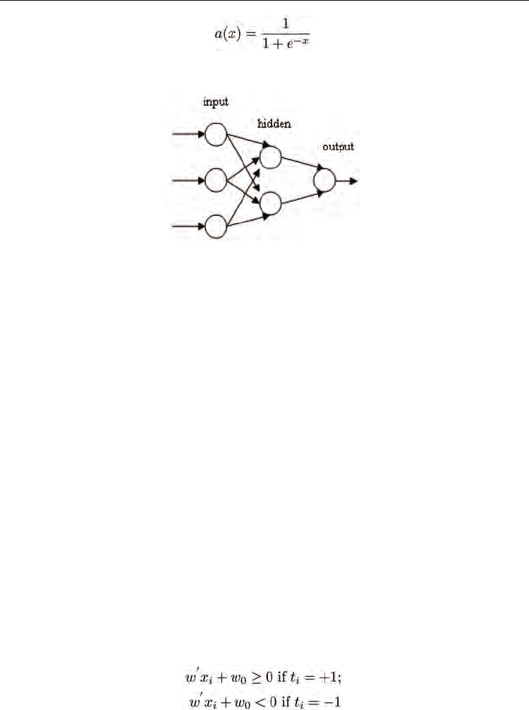
3.4 Neural networks

A neural network is structured as a set of interconnected identical units (neurons). The

interconnections are used to send signals from one neuron to the other. In addition, the

interconnections have weights to enhance the delivery among neurons (Marques de Sa,

2001). The neurons are not powerful by themselves, however, when connected to others

they can perform complex computations. Weights on the interconnections are updated

when the network is trained, hence significant interconnection play more role during the

testing phase. Figure 3 depicts an example of neural network. The neural network in the

figure consists of one input layer, one hidden layer, and one output layer. Since

interconnections do not loop back or skip other neurons, the network is called feedforward.

The power of neural networks comes from the nonlinearity of the hidden neurons. In

consequence, it is signi_cant to introduce nonlinearity in the network to be able to learn

complex mappings. The commonly used function in neural network research is the sigmoid

function, which has the form (Massey et al., 2003)

Machine Learning

194

Although competitive in learning ability, the fitting of neural network models requires some

experience, since multiple local minima are standard and delicate regularization is required.

Fig. 3. Neural Network.

3.5 Random forests

Random forests are classi_ers that combine many tree predictors, where each tree depends

on the values of a random vector sampled independently. Furthermore, all trees in the forest

have the same distribution (Breiman, 2001). In order to construct a tree we assume that n is

the number of training observations and p is the number of variables (features) in a training

set. In order to determine the decision node at a tree we choose k << p as the number of

variables to be selected. We select a bootstrap sample from the n observations in the training

set and use the rest of the observations to estimate the error of the tree in the testing phase.

Thus, we randomly choose k variables as a decision at a certain node in the tree and

calculate the best split based on the k variables in the training set. Trees are always grown

and never pruned compared to other tree algorithms.

Random forests can handle large numbers of variables in a data set. Also, during the forest

building process they generate an internal unbiased estimate of the generalization error. In

addition, they can estimate missing data well. A major drawback of random forests is the

lack of reproducibility, as the process of building the forest is random. Further, interpreting

the final model and subsequent results is difficult, as it contains many independent

decisions trees.

3.6 Support vector machines

Support Vector Machines (SVM) are one of the most popular classifiers these days. The idea

here is to find the optimal separating hyperplane between two classes by maximizing the

margin between the classes closest points. Assume that we have a linear discriminating

function and two linearly separable classes with target values +1 and -1. A discriminating

hyperplane will satisfy:

Now the distance of any point x to a hyperplane is │ w’x

│ / ║ w ║ and the distance to

the origin is │ w

│ / ║ w ║. As shown in Figure 4 the points lying on the boundaries are

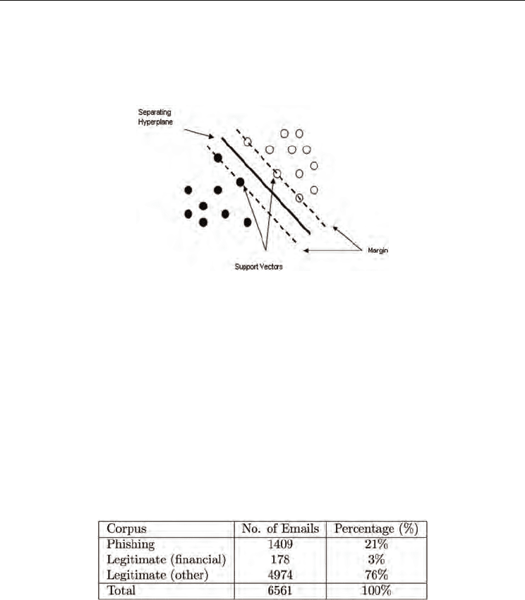
Hardening Email Security via Bayesian Additive Regression Trees

195

called support vectors, and the middle of the margin is the optimal separating hyperplane

that maximizes the margin of separation (Marques de Sa, 2001).

Though SVMs are very powerful and commonly used in classification, they suffer from

several drawbacks. They require high computations to train the data. Also, they are

sensitive to noisy data and hence prone to overfitting.

Fig. 4. Support Vector Machines.

4. Quantitative evaluation

4.1 Phishing dataset

The phishing dataset constitutes of 6561 raw emails. The total number of phishing emails in

the dataset is 1409 emails. These emails are donated by (Nazario, 2007) covering many of the

new trends in phishing and collected between August 7, 2006 and August 7, 2007. The total

number of legitimate email is 5152 emails. These emails are a combination of financial-

related and other regular communication emails. The financial-related emails are received

from financial institutions such as Bank of America, eBay, PayPal, American Express, Chase,

Amazon, AT&T, and many others. As shown in Table 1, the percentage of these emails is 3%

of the complete dataset. The other part of the legitimate set is collected from the authors'

mailboxes. These emails represent regular communications, emails about conferences and

academic events, and emails from several mailing lists.

Table 1. Corpus description.

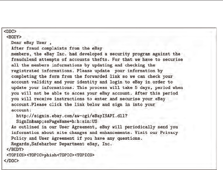
4.1.1 Data standardization, cleansing, and transformation

The analysis of emails consists of two steps: First, textual analysis, where text mining is

performed on all emails. In order to get consistent results from the analysis, one needs to

standardize the studied data. Therefore, we convert all emails into XML documents after

stripping all HTML tags and email header information. Figure 5 shows an example of a

phishing email after the conversions. Text mining is performed using the text-miner

software kit (TMSK) provided by (Weiss et al., 2004). Second, structural analysis. In this step

Machine Learning

196

we analyze the structure of emails. Specifically, we analyze links, images, forms, javascript

code and other components in the emails.

Fig. 5. Phishing email after conversion to XML.

Afterwards, each email is converted into a vector

= 〈x

, x

, ..., x

〉, where x

, ..., x

are the

values corre- sponding to a specific feature we are interested in studying (Salton & McGill,

1983). Our dataset consists of 70 continuous and binary features (variables) and one binary

response variable, which indicates that email is phishing=1 or legitimate=0. The first 60

features represent the frequency of the most frequent terms that appear in phishing emails.

Choosing words (terms) as features is widely applied in the text mining literature and is

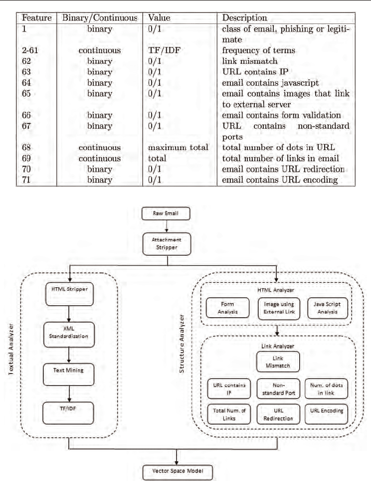
referred to as “bag-of-words”. In Table 2 we list both textual and structural features used in

the dataset. As shown in Figure 6, we start by striping all attachments from emails in order to

facilitate the analysis of emails. The following subsections illustrate the textual and

structural analysis in further details.

4.1.2 Textual analysis

As we mentioned earlier we start by stripping all attachments from email messages. Then, we

extract the header information of all emails keeping the email body. Afterwards, we extract

the html tags and elements from the body of the emails, leaving out the body as plain text.

Now, we standardize all emails in a form of XML documents. The <DOC> </DOC> tags

indicate the beginning and ending of a document respectively. The <BODY> </BODY> tags

indicate the starting and ending of an email body respectively. The <TOPICS> </TOPICS>

tags indicate the class of the email, whether it is phish or legit (see Figure 5).

Hardening Email Security via Bayesian Additive Regression Trees

197

Table 2. Feature description.

Fig. 6. Building the phishing dataset.

Thus, we filter out stopwords from the text of the body. We use a list of 816 commonly used

English stopwords. Lastly, we find the most frequent terms using TF/IDF (Term Frequency

Inverse Document Frequency) and choose the top 60 most frequent terms that appear in

Machine Learning

198

phishing emails. TF/IDF calculates the number of times a word appears in a document

multiplied by a (monotone) function of the inverse of the number of documents in which the

word appears. In consequence, terms that appear often in a document and do not appear in

many documents have a higher weight (Berry, 2004).

4.1.3 Structural analysis

Textual analysis generates the first 60 features in the dataset and the last 10 features are

generated using structural analysis. Unlike textual analysis, here we only strip the

attachments of emails keeping HTML tags and elements for further analysis. First, we

perform HTML analysis, in which we analyze form tags, javascript tags, and image tags.

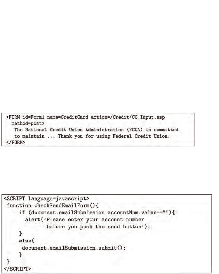
Legitimate emails rarely contain form tags that validate the user input. Phishing emails, on

the other hand, use this techniques to validate victims' credentials before submitting them to

the phishing site. In consequence, if an email contains a form tag, then the corresponding

feature in the dataset is set to 1, otherwise it is set to 0. Figure 7 shows an example of a

Federal Credit Union phish which contains a form tag.

Fig. 7. Form validation in phishing email.

Similarly, legitimate emails rarely contain javascript, however, phishers use javascript to

validate users input or display certain elements depending on the user input. If the email

contains javascript, then the corresponding feature in the dataset is set to 1, otherwise it is

set to 0. Figure 8 shows an example of javascript that is used by a phisher to validate the

victims account number.

Fig. 8. Javascript to validate account number.

Spammers have used images that link to external servers in their emails, also dubbed as Web

beacons, to verify active victims who preview or open spam emails. Phishers also have been

following the same technique to verify active victims and also to link to pictures from

legitimate sites. We analyze emails that contain image tags that link to external servers. If the

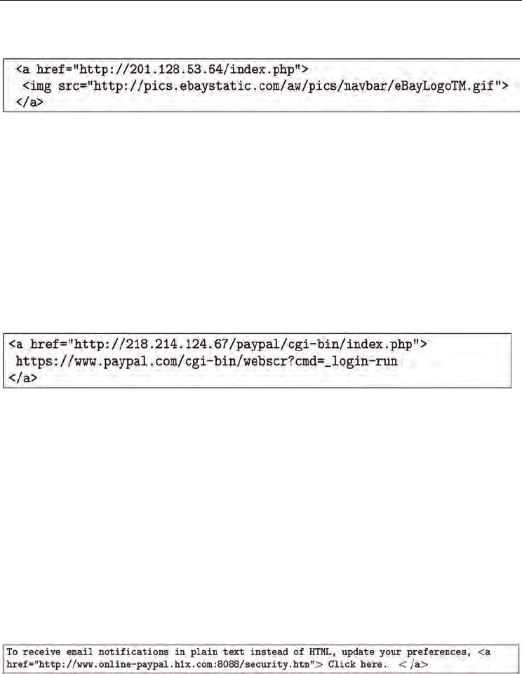
Hardening Email Security via Bayesian Additive Regression Trees

199

email contains such an image, then the corresponding feature in the dataset is set to 1,

otherwise it is set to 0. Figure 9 shows an example of a image tag with an external link.

Fig. 9. Image linking to an external server.

The second part in structural analysis involves the link analysis process. Here we analyze

links in emails. It is well known that phishers use several techniques to spoof links in emails

and in webpages as well to trick users into clicking on these links. When analyzing links we

look for link mismatch, URL contains IP address, URL uses non-standard ports, the

maximum total number of dots in a link, total number of links in an email, URL redirection,

and URL encoding. In what follows we describe these steps in more details.

When identifying a link mismatch we compare links that are displayed to the user with their

actual destination address in the <a href> tag. If there is a mismatch between the

displayed link and the actual destination in any link in the email, then the corresponding

feature in the dataset is set to 1, otherwise, it is set to 0. Figure 10 shows an example of a

PayPal phish, in which the phisher displays a legitimate Paypal URL to the victim; however,

the actual link redirects to a Paypal phish.

Fig. 10. URL mismatch in link.

A commonly used technique, but easily detected even by naive users, is the use of IP

addresses in URLs (i.e. unresolved domain names). This has been and is still seen in many

phishing emails. It is unlikely to see unresolved domain names in legitimate emails;

however, phishers use this technique frequently, as it is more convenient and easier to setup

a phishing site. If the email contains a URL with an unresolved name, then the

corresponding feature in the dataset is set to 1, otherwise, it is set to 0. Phishers often trick

victims by displaying a legitimate URL and hiding the unresolved address of the phishing

site in the <a href> tag as shown in the example in Figure 10.

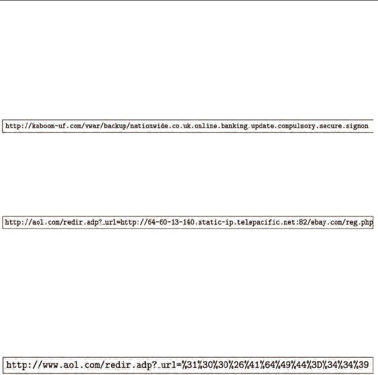
Since phishing sites are sometimes hosted at compromised sites or botnets, they use non-

standard port numbers in URLs to redirect the victim's traffic. For example instead of using

port 80 for http or port 443 for https traffic, they use different port numbers. If the email

contains a URL that redirects to a non-standard port number, then the corresponding

feature in the dataset is set to 1, otherwise it is set to 0. Figure 11 shows an example of a

phishing URL using a non-standard port number.

Fig. 11. Phishing URL using non-standard port number.

We count the number of links in an email. Usually, phishing emails contain more links

compared to legitimate ones. This is a commonly used technique in spam detection, where

messages that contain a number of links more than a certain threshold are filtered as spam.

Machine Learning

200

However, since phishing emails are usually duplicate copies of legitimate ones, this feature

might not help in distinguishing phishing from financial-related legitimate emails; however,

it helps in distinguishing phishing from other regular legitimate messages.

Since phishing URLs usually contain multiple sub-domains so the URL looks legitimate, the

number of dots separating sub-domains, domains, and TLDs in the URLs are usually more

than those in legitimate URLs. Therefore, in each email we find the link that has the

maximum number of dots. The maximum total number of dots in a link in an email thus is

used as a feature in the dataset. Figure 12 shows an example of a Nationwide spoof link.

Note the dots separating different domains and sub-domains.

Fig. 12. Number of dots in a Nationwide spoof URL.

Phishers usually use open redirectors to trick victims when they see legitimate site names in

the URL. Specifically, they target open redirectors in well known sites such as aol.com,

yahoo.com, and google.com. This technique comes handy when combined with other

techniques, especially URL encoding, as naive users will not be able to translate the

encoding in the URL. Figure 13 shows an example of an AOL open redirector.

Fig. 13. Open redirector at AOL.

The last technique that we analyze here is URL encoding. URL encoding is used to transfer

characters that have a special meaning in HTML during http requests. The basic idea is to

replace the character with the “%” symbol, followed by the two-digit hexadecimal

representation of the ISO-Latin code for the character. Phishers have been using this

approach to mask spoofed URL and hide the phony addresses of these sites. However, they

encode not only special characters in the URL, but also the complete URL. As we mentioned

earlier, when this approach is combined with other techniques, it makes the probability of

success for the attack higher, as the spoofed URL looks more legitimate to the naive user.

Figure 14 shows an example of URL encoding combined with URL redirection.

Fig. 14. URL encoding combined with URL redirection.

Figure 6 depicts a block diagram of the approach used in building the dataset. It shows both

textual and structural analysis and the procedures involved therein.

4.2 Evaluation metrics

We use the area under the receiver operating characteristic (ROC) curve (AUC) to measure

and compare the performance of classifiers. According to (Huang & Ling, 2005), AUC is a

better measure than accuracy when comparing the performance of classifiers. The ROC

curve plots false positives (FP) vs. true positives (TP) using various threshold values. It

compares the classifiers' performance across the entire range of class distributions and error

costs (Huang & Ling, 2005).

Let N

denote the total number of legitimate emails, and N

denote the total number of

phishing emails. Now, let n

→

be the number of legitimate messages classified as legitimate,

Hardening Email Security via Bayesian Additive Regression Trees

201

→

be the number of legitimate messages misclassified as phishing, n

→

be the number of

phishing messages misclassified as legitimate, and n

→

be the number of phishing messages

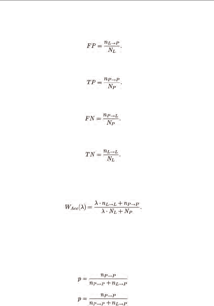
classified as phishing. False positives are legitimate emails that are classified as phishing,

hence the false positive rate (FP) is denoted as:

(8)

True positives are phishing emails that are classified as phishing, hence the true positive rate

(TP) is denoted as:

(9)

False negatives are phishing emails that are classified as legitimate, hence the false negative

rate (FN) is denoted as:

(10)

True negatives are legitimate emails that are classified as legitimate, hence the true negative

rate (TN) is denoted as:

(11)

Further we evaluate the predictive accuracy of classifiers, by applying the weighted error

Err

) measure proposed in (Sakkis et al., 2003) and (Zhang et al., 2004). We test the

classifiers using

= 1 that is when legitimate and phishing emails are weighed equally.

Hence the weighted accuracy (W

Acc

), which is 1 - W

Err

(

), can be calculated as follows

(12)

In addition, we use several other measures to evaluate the performance of classifiers. We use

the phishing recall(r), phishing precision(p), and phishing f

measures. According to (Sakkis et

al., 2003), spam recall measures the percentage of spam messages that the filter manages to

block (filter's effectiveness). Spam precision measures the degree to which the blocked

messages are indeed spam (filter's safety). F-measure is the weighted harmonic mean of

precision and recall. Here we use f

when recall and precision are evenly weighted. For the

above measures, the following equations hold

(13)

(14)

Machine Learning

202

(15)

We use the AUC as the primary measure, as it allows us to gauge the trade off between the

FP and TP rates at different cut-off points. Although the error rate W

Err

(or accuracy) has

been widely used in comparing classifiers’ performance, it has been criticized as it highly

depends on the probability of the threshold chosen to approximate the positive classes. Here

we note that we assign new classes to the positive class if the probability of the class is

greater than or equal to 0.5 (threshold=0.5). In addition, in (Huang & Ling, 2005) the authors

prove theoretically and empirically that AUC is more accurate than accuracy to evaluate

classi_ers' performance. Moreover, although classifiers might have different error rates,

these rates may not be statistically significantly different. Therefore, we use the Wilcoxon

signed-ranks test (Wilcoxon, 1945) to compare the error rates of classifiers and find whether

the di_erences among these accuracies is significant or not (Demšar, 2006).

4.3 Experimental studies

We optimize the classifiers’ performance by testing them using different input parameters.

In order to find the maximum AUC, we test the classifiers using the complete dataset

applying different input parameters. Also, we apply 10-fold-cross-validation and average the

estimates of all 10 folds (sub-samples) to evaluate the average error rate for each of the

classifiers, using the 70 features and 6561 emails. We do not perform any preliminary

variable selection since most classifiers discussed here can perform automatic variable

selection. To be fair, we use L1-SVM and penalized LR, where variable selection is

performed automatically.

We test NNet using different numbers of units in the hidden layer (i.e. different sizes (s))

ranging from 5 to 35. Further, we apply different weight decays (w) on the interconnections,

ranging from 0.1 to 2.5. We find that a NNet with s = 35 and w = 0.7 achieves the maximum

AUC of 98.80%.

RF is optimized by choosing the number of trees used. Specifically, the number of trees we

consider in this experiment is between 30 and 500. When using 50 trees on our dataset, RF

achieves the maximum AUC of 95.48%.

We use the L1-SVM C-Classification machine with radial basis function (RBF) kernels. L1-

SVM can automatically select input variables by suppressing parameters of irrelevant

variables to zero. To achieve the maximum AUC over different parameter values, we

consider cost of constraints violation values (i.e. the “c” constant of the regularization term

in the Lagrange formulation) between 1 and 16, and values of the γ parameter in the kernels

between 1 ×10

-8

and 2. We find that γ= 0.1 and c = 12 achieve the maximum AUC of 97.18%.

In LR we use penalized LR and apply different values of the lambda regularization

parameter under the L2 norm, ranging from 1 × 10

-8

to 0.01. In our dataset

= 1 × 10

-4

achieves the maximum AUC of 54.45%.

We use two BART models; the first is the original model and as usual, we refer to this as

“BART”. The second model is the one we modify so as to be applicable to classification,

referred to as “CBART”. We test both models using different numbers of trees ranging from

30 to 300. Also, we apply different power parameters for the tree prior, to specify the depth

of the tree, ranging from 0.1 to 2.5. We find that BART with 300 trees and power = 2.5

achieves the maximum AUC of 97.31%. However, CBART achieves the maximum AUC of

99.19% when using 100 trees and power = 1.