Marulanda J.M. (ed.) Electronic Properties of Carbon Nanotubes
Подождите немного. Документ загружается.

Quantum Calculation in Prediction
the Properties of Single-Walled Carbon Nanotubes
585
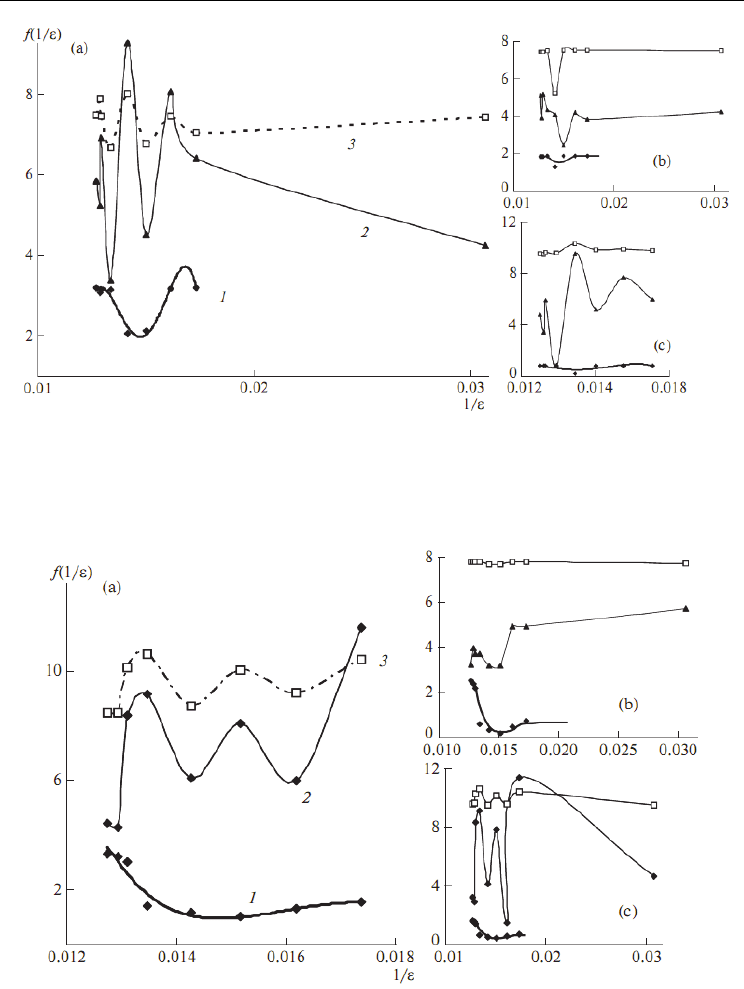
Fig. 3. The natural logarithms of the potential energy (1), intensity (2), and frequency (3) of
three normal modes (a) 1, (b) 61, (c) 66 versus inverse of dielectric constant for nanotube (3,
0) with D3d point group by AM1 calculation (Lee et al., 2009)
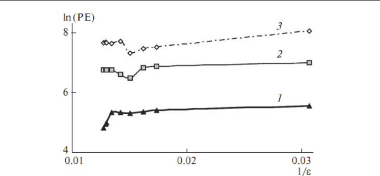
Fig. 4. The logarithms of the potential energy (1), intensity (2), and frequency (3) of three
normal modes (a) 1, (b) 131, (c) 138 versus inverse of dielectric constant for nanotube (4, 0)
with D4d point group by AM1 calculation (Lee et al., 2009)
Electronic Properties of Carbon Nanotubes
586
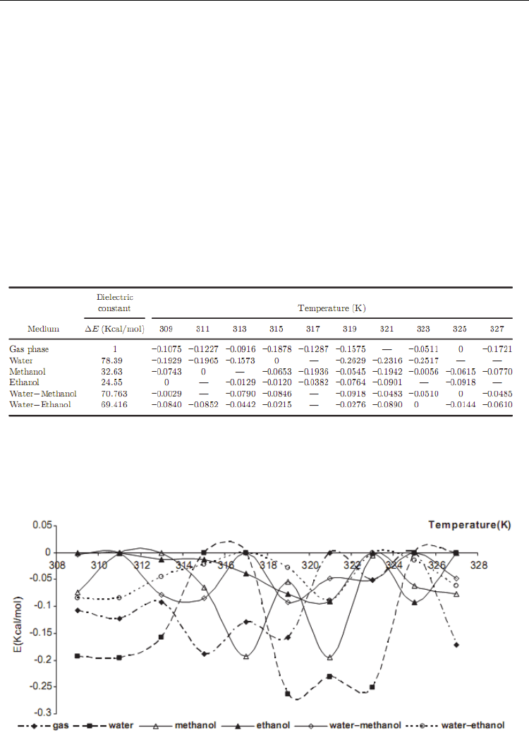
Fig. 5. The logarithms of the potential energy (PE) of three different zigzag nanotubes (1)
D3d, (2) D4d, (3) D5d versus inverse of dielectric constant by MC simulations (Lee et al.,
2009)
2.7 Potential energy dependence on the dielectrics of zigzag nanotubes
In Fig. 3 three line of potential energy for three nanotubes are shown by the Monte Carlo
calculation versus dielectric constants. For D3d symmetric nanotube, the logarithm of
potential energy increases as the dielectric constant reduces from 78.39 up to 76.10 while the
D4d and D5d symmetries show an unchanged potential energy in this region. Beyond this
point, the potential energy of D4d and D5d nanotubes drop and rise again to be in a new
equilibrium, whereas the potential energy of the D3d mostly constant as the dielectric
constant decreases. There are some changing in the energy in variable with the dielectrics
above 60, and by decreasing the dielectrics the energy of three nanotubes goes toward
constant variables. Similar trends between three figures and there are very good agreement
with ab initio calculation in the Table 1.
3. Stability of SWCNTs: Solvents and temperature effects by molecular
dynamics simulation and quantum mechanics calculations
Structural properties of solvents such as water, methanol, and ethanol surrounding single-
walled carbon nanotube (SWCNT) and mixtures of them as well have an effects on the
relative energies and dipole moment values. Because some of the physicochemical
parameters are elated to structural properties of SWCNT, the different force fields can be
examined to determine energy and other types of geometrical parameters, on the particular
SWCNT. Because of the differences among force fields, the energy of a molecule calculated
using two different force fields will not be the same. The structure of SWCNT as well as its
dipole moments and relative energies has been studied by molecular dynamics simulation
and quantum mechanics calculations (Monajjemi et al., 2010). The term “Ab Initio" is given to
computations which are derived directly from theoretical principles, with no inclusion of
experimental data. The most common type of ab initio calculation is called a Hartree-Fock
(HF) calculation, in which the primary approximation is called the central field
approximation. A method, which avoids making the HF mistakes in the first place, is called

Quantum Calculation in Prediction
the Properties of Single-Walled Carbon Nanotubes
587
Quantum Monte Carlo (QMC). There are several favors of QMC variational, diffusion, and
Green's functions. These methods work with an explicitly correlated wave function and
evaluate integrals numerically using a Monte Carlo integration. These calculations can be
very time consuming, but they are probably the most accurate methods known today. In
general, ab initio calculations give very good qualitative results and can give increasingly
accurate quantitative results as the molecules in question become smaller (Monajjemi et al.,
2008a). In general, there are three steps in carrying out any quantum mechanical calculation.
First, prepare a molecule with an appropriate starting geometry. Second, choose a
calculation method and its associated options. Third, choose the type of calculation with the
relevant options and finally, analyze the results. We will give a short detail of computational
method in the following section.
3.1 Molecular mechanics (Monte Carlo simulation)
The Metropolis implementation of the Monte Carlo algorithm has been developed by
studying the equilibrium thermodynamics of many-body systems. Choosing small trial
moves, the trajectories obtained applying this algorithmagree with those obtained by
Langevin's dynamics (Tiana et al., 2007). This is understandable because the Monte Carlo
simulations always detect the so-called “important phase space" regions which are of low
energy (Liu & Monson, 2005). Because of imperfections of the force field, this lowest energy
basin usually does not correspond to the native state in most cases, so the rank of native
structure in those decoys produced by the force field itself is poor. In density function
theory the exact exchange (HF) for a single determination is replaced by a more general
expression of the exchange correlation functional, which can include terms accounting for
both exchange energy and the electron correlation, which is omitted from HartreeFock
theory:
E
ks
=+<hp>+1/2<P
j
()>+E
(
)
+E
C(
)
where E
(
)
is the exchange function and E
C(
)
is the correlation functional. The correlation
function of Lee et al. includes both local and nonlocal terms (Lee et al., 1988).
3.2 Langevin dynamics (LD) simulation
The Langevin equation is a stochastic differential equation in which two force terms have
been added to Newton's second law to approximate the effects of neglected degrees of
freedom (Wang & Skeel, 2003). These simulations can be much faster than molecular
dynamics. The molecular dynamics method is useful for calculating the time-dependent
properties of an isolated molecule. However, more often, one is interested in the properties
of a molecule that is interacting with other molecules.
3.3 Effect of differenct solvents of temperatures of SWCNTusing molecular dynamics
simulation and quantum mechanics calculations
Difference in force field is illustrated by comparing the energy calculated by using force
fields, MM+, Amber, and Bio+. The quantum mechanics (QM) calculations were carried out
with the GAUSSIAN98 program based on HF/3-21G level. In the Gaussian program a
simple approximation is used in which the volume of the solute is used to compute the
radius of a cavity which forms the hypothetical surface of the molecule (Witanowski et al.,
2002; Mora-Diez et al., 2006). The structures in gas phase and different solvent media such as
Electronic Properties of Carbon Nanotubes
588
water, methanol, ethanol, and mixtures of them have been compared. The structure of
SWCNT as well as its dipole moments and relative energies has been studied by molecular
dynamics simulation and quantum mechanics calculations within the Onsager self-
consistent reaction field (SCRF) model using a Hartree-Fock method (HF) at the HF/3-21G
level and the structural stability of considered nanotube in different solvent media and
temperature (between 309K and 327K) have been compared and analyzed.
Since the influence between a molecule in solution and its medium can describe most simply
by using Onsager model, in this model we have assumed that the solute is placed in a
spherical cavity inside the solvent. The latter is described as a homogeneous, polarizable
medium of dielectric constant. We started our studies with HF/3-21G gas phase geometry
and water, methanol and ethanol surrounding SWCNT and mixtures of them as well. The
results obtained from Onsager model calculations are illustrated using the energy difference
between these conformers which are quite sensitive to the polarity of the surrounding
solvent. The solvent effect has been calculated using SCRF model. According to this method,
the total energy of solute and solvent, which depends on the dielectric constant has been
listed in Table 2.
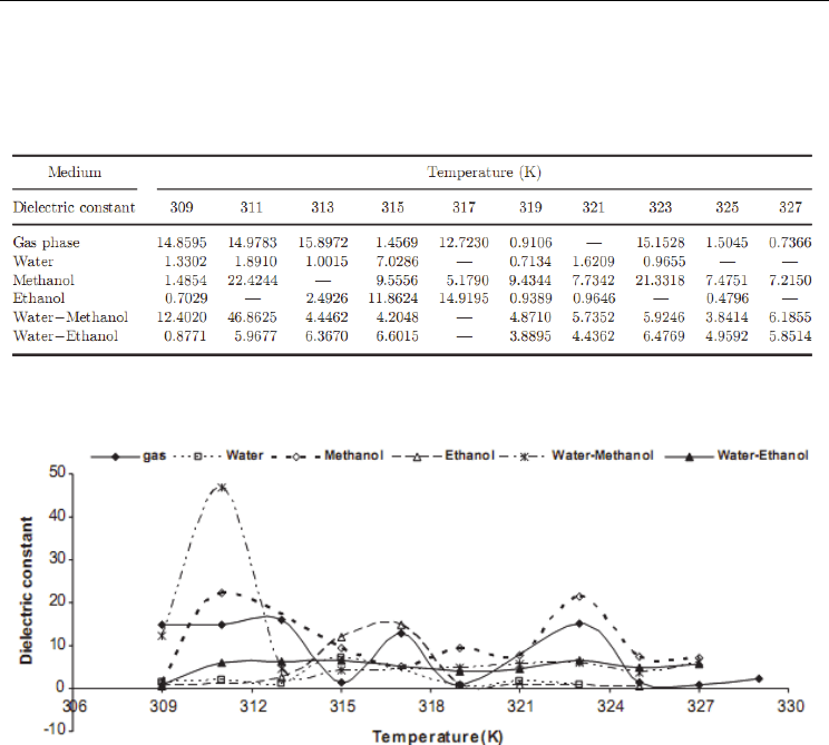
Table 2. Theoretical relative energies at different temperature and dielectric constant
These energies have been compared with the gas phase total energy CNT at the HF/3-21G
level of theory and different solvents, and the graph of energy values versus dielectric
constant of different solvents has been displayed at considered temperatures in Fig. 6.
Fig. 6. The relative energy values at different temperatures in different solvents.
Quantum Calculation in Prediction
the Properties of Single-Walled Carbon Nanotubes
589
Since the solute dipole moment induces a dipole moment in opposite direction in the
surrounding medium, polarization of the medium in turn polarizes the charge distribution
in the solvent. The dipole moment value of SWCNT in different solvent media and at
different temperatures has been reported in Table 3.
Table 3. Theoretical dipole moment values at different temperatures
Fig. 7. The dipole moment values at different temperatures
One much more practical approach consists of calculating the molecular volume as defined
through the contour of constant electron density, equating this (nonspherical) molecular
volume to the radius of an ideally spherical cavity, and adding a constant increment for the
closest possible approach of solvent molecules. This latter approach was used in Gaussian
when the volume keyword was being used. In this work, we studied the structural
properties of water, methanol, and ethanol surrounding SWCNT and mixtures of them as
well as using molecular dynamics simulations. We used different force fields for
determination of energy and other types of geometrical parameters, on the particular
SWCNT. Because of the differences among force fields, the energy of a molecule calculated
using two different force fields will not be the same. So, it is not reasonable to compare the
energy of one molecule calculated with a particular force field with the energy of another
molecule calculated using a different force field. In this study difference in force field
illustrated by comparing the energy calculated by using force fields, MM+, AMBER, and
BIO+. Theoretical energy values using difference force fields which are the combination of
attraction van der Waals forces due to dipole-dipole interactions and empirical repulsive
forces due to Pauli repulsion have been demonstrated in Table 4 and Fig. 8.

Electronic Properties of Carbon Nanotubes
590
Table 4. Theoretical energy values using different force fields
Fig. 8. The energy values using different force fields
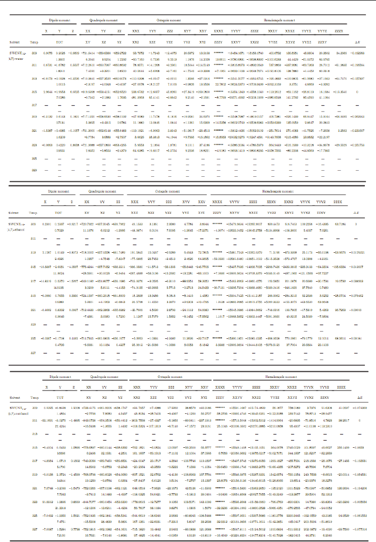
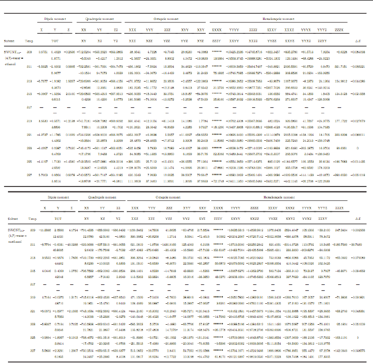
The result of the calculated dipole moment, quadrupole moment, octapole moment, and
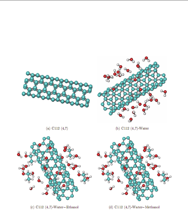
hexadecapole moment values of SWCNT has been reported in Table 5, and optimized
structures of nanotube in different media are shown in Fig. 9.
Quantum Calculation in Prediction
the Properties of Single-Walled Carbon Nanotubes
591
Electronic Properties of Carbon Nanotubes
592
Table 5. The calculated dipole moment, quadrupole moment, octapole moment, and
hexadecapole moment values of SWCNT
4. NMR and IR theoretical study on the interaction of doping metal with
carbon nanotube (CNT)
Numerous electrical measurements on SWCNT ensembles have revealed that chemical
doping by donors (Li, K, Cs, or Rb) or acceptors (Br
2
, I
2
, or acids) decreases the room
temperature electrical resistance by up to two orders of magnitude at saturation doping
(Kaaoui et al., 1999; Coluci et al. 2006). The important problem is metals passing through
cells membrane. Because, there are barriers for them passing through protein canals in cells
membrane. Additionally, upon interaction, changes in activity, stability, and solubility ions
compatibility may occur in cells. A lot of studies are for replacing protein canals into cells
membrane for passing proteins, drug and ions of metal. Therefore the presence of the
SWCNT and its consequences to the biological activity of ions metal are of high impact in
Quantum Calculation in Prediction
the Properties of Single-Walled Carbon Nanotubes
593
the development of biosensors, immunoassays and drug delivery systems (Zhang et al.,
2005; Ganjali et al., 2006). This work, we used armchair carbon nanotube (5, 5) and (6, 6).
Indeed, vibrational frequencies of finite-length carbon nanotubes were recently examined
(Tagmatarchris & Prato, 2004) and another result of 319.9 cm
–1
is consistent with oscillations
along the radial directions (radial modes), although it cannot be assessed accurately due to
the sensitivity to the number of rings (Yumura et al., 2005). We suggest that SWCNT
intercalate into cells membrane replacing protein canals and are studying passing metal ions
(Na, Mg, Al, and Si) in length of SWCNT by Quantum Mechanics (QM).
Fig. 9. Optimized structures of nanotube in different media
4.1 Computational details
The geometry optimizations were performed using an all-electron linear combination of
atomic orbitals Hatree–Fock (HF) and density functional theory (DFT) calculations using the
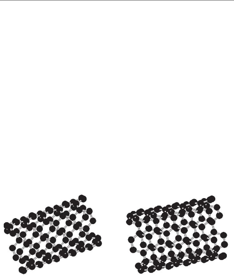
Gaussian A7 package. SWCNTs (100–120) from kind of armchair carbon nanotubes (5, 5)
and (6, 6) show in Fig. 10. We are interested in the structural features of single-walled
carbon nanotube (SWCNT) in the ground state an atomic and amino acids (His and Ser). In
HF theory the energy has from:
Electronic Properties of Carbon Nanotubes
594
E
ks
=+<hp>+1/2<P
j
()>-1/2<P
k
()>
where ν is the nuclear repulsion energy, ρ is the density matrix,
〈hp〉 is the one electron
(kinetic plus potential energy). 1/2
〈P
j
(ρ)〉 is the classical coulomb repulsion of the electrons
and –1/2
〈P
k
(ρ)〉 is the exchange energy resulting from the quantum (fermions) nature of
electrons.
In density function theory the exact exchange (HF) for a single determinant is replaced by a
more general expression the exchange correlation functional, which can include terms
accounting for both exchange energy and the electron correlation, which is omitted from
Hartree–Fock theory:
E
ks
=+<hp>+1/2<P
j
()>+E
(
)
+E
C(
)
where, E
(
)
is the exchange function and E
C(
)
is the correlation functional. The correlation
function of Lee, Yang, and Parr is includes both local and non-local term (Kar et al., 2006).
The optimizations of solids are carried out including exchange and correlation contributions
using Becks three parameters hybrid and Lee–Yang–Parr (LYP) correlation [B3LYP];
including both local and non-local terms with the program Gaussian A7 package (Lee et al.,
1988; Becke, 1993; Becke, 1997).
Compared to Raman spectroscopy, much less information about the vibration properties of
carbon nanotubes can be gained from IR spectra. This limitation mainly results from the
strong absorption of SWCNTs in the IR range. Accurate predictions of molecular response
properties to external fields are of general significance in various areas of chemical physics.
This especially refers to the second-order magnetic response properties (NMR), since the
magnetic resonance based techniques have gained substantial importance in chemistry and
biochemistry that NMR data shown with two parameters isotropic (σ
iso
) and an isotropic
(σ
aniso
) shielding.
Fig. 10. The optimized configuration Side-view SWCNT: C
100
(a) and C
120
(b)
4.2 Interaction of Na, Mg, Al, Si with Carbon Nanotube (CNT): NMR and IR Study
The B3LYP and HF by 6–31G and 6–31G* calculaion for the molecular SWCNT models with
Na, Mg, Al, and Si considered were validated by the calculated 13C and 1H NMR shifts and
thermodynamic properties of an open-ended SWCNT (5, 5) and (6, 6) molecular systems
(Monajjemi et al., 2009). The total energy (Etotal) of this interaction is listed in Table 6, which
the Etotal increase to converge with an increasing carbon number.