Kannan R., Vempala S. Spectral Algorithms
Подождите немного. Документ загружается.


Chapter 4
Recursive Spectral
Clustering
In this chapter, we study a spectral algorithm for partitioning a graph. The key
algorithmic ingredient is a procedure to find an approximately minimum con-
ductance cut. This cutting procedure is used recursively to obtain a clustering
algorithm. The analysis is based on a natural bicriteria measure for assessing
the quality of a clustering and makes no probabilistic assumptions on the input
data. We begin with an important definition. Given a graph G = (V, E), with
nonnegative edge weights a
ij
, for a subset of vertices S, we let a(S) denote the
total weight of edges incident to vertices in S. Then the conductance of a subset
S is
φ(S) =
P
i∈S,j6∈S
a
ij
min{a(S), a(V \S)}
,
and the conductance of the graph is
φ = min
S⊂V
φ(S).
4.1 Approximate minimum conductance cut
The following simple algorithm takes a weighted graph (or weighted adjacency
matrix) as input and outputs a cut of the graph.
37

38 CHAPTER 4. RECURSIVE SPECTRAL CLUSTERING
Algorithm: Approximate-Cut
1. Normalize the adjancency matrix so each row sum is 1.
2. Find the second largest eigenvector of this matrix.
3. Order the vertices according their components in this
vector.
4. Find the minimum conductance cut among cuts given by this
ordering.
The following theorem bounds the conductance of the cut found by this
heuristic with respect to the minimum conductance. This theorem plays an im-
portant role in the analysis of Markov chains, where conductance is often easier
to estimate than the desired quantity, the spectral gap. The latter determines
the mixing rate of the Markov chain. Later in this chapter, we will use this
cutting procedure as a tool to find a clustering.
Theorem 4.1. Suppose B is a N × N matrix with non-negative entries with
each row sum equal to 1 and suppose there are positive real numbers π
1
, π
2
, . . . π
N
summing to 1 such that π
i
b
ij
= π
j
b
ji
for all i, j. If v is the right eigenvector
of B corresponding to the second largest eigenvalue λ
2
, and i
1
, i
2
, . . . i
N
is an
ordering of 1, 2, . . . N so that v
i
1
≥ v
i
2
. . . ≥ v
i
N
, then
min
S⊆{1,2,...N}
P
i∈S,j /∈S
π
i
b
ij
min(
P
i∈S
π
i
,
P
j /∈S
π
j
)
≥ 1 − λ
2
≥
1
2
min
l,1≤l≤N
P
1≤u≤l;l+1≤v≤N
π
i
u
b
i
u
i
v
min(
P
1≤u≤l
π
i
u
,
P
l+1≤v≤N
π
i
v
)
2
We note here that the leftmost term above is just the conductance of the
graph with weights b
ij
, while the rightmost term is the square of the minimum
conductance of cuts along the ordering given by the second eigenvector of the
of the normalized adjacency matrix. Since the latter is trivially at least as large
as the square of the overall minimum conductance, we get
min conductance ≥ 1 − λ
2
≥
1
2
(min conductance)
2
.
Proof (of Theorem 4.1). We first evaluate the second eigenvalue. Towards
this end, let D
2
= diag(π). Then, from the time-reversibility property of B,
we have D
2
B = B
T
D
2
. Hence Q = DBD
−1
is symmetric. The eigenvalues of
B and Q are the same, with their largest eigenvalue equal to 1. In addition,
π
T
D
−1
Q = π
T
D
−1
and therefore π
T
D
−1
is the left eigenvector of Q corre-
sponding to the eigenvalue 1. So we have,
λ
2
= max
π
T
D
−1
x=0
x
T
DBD
−1
x
x
T
x

4.1. APPROXIMATE MINIMUM CONDUCTANCE CUT 39
Thus, substituting y = D
−1
x, we obtain
1 − λ
2
= min
π
T
D
−1
x=0
x
T
D(I −B)D
−1
x
x
T
x
= min
π
T
y=0
y
T
D
2
(I −B)y
y
T
D
2
y
The numerator can be rewritten:
y
T
D
2
(I −B)y = −
X
i6=j
y
i
y
j
π
i
b
ij
+
X
i
π
i
(1 − b
ii
)y
2
i
= −
X
i6=j
y
i
y
j
π
i
b
ij
+
X
i6=j
π
i
b
ij
y
2
i
+ y
2
j
2
=
X
i<j
π
i
b
ij
(y
i
− y
j
)
2
Denote this final term by E(y, y). Then
1 − λ
2
= min
π
T
y=0
E(y, y)
P
i
π
i
y
2
i
To prove the first inequality of the theorem, let (S,
¯
S) be the cut with the
minimum conductance. Define a vector w as follows
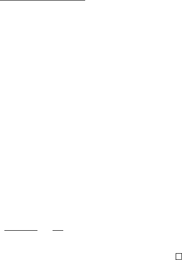
w
i
=
q
1
P
u
a(u)
π(
¯
S)
π(S)
if i ∈ S
−
q
1
P
u
a(u)
π(S)
π(
¯
S)
if i ∈
¯
S
It is then easy to check that
P
i
π
i
w
i
= 0 and that
φ(S) ≥
E(w, w)
P
i
π
i
w
2
i
≥ 1 − λ
2
Hence we obtain the desired lower bound on the conductance.
We will now prove the second inequality. Suppose that the minimum above
is attained when y is equal to v. Then Dv is the eigenvector of Q corresponding
to the eigenvalue λ
2
and, v is the right eigenvector of B corresponding to λ
2
.
Our ordering is then with respect to v in accordance with the statement of the
theorem. Assume that, for simplicity of notation, the indices are reordered (i.e.
the rows and corresponding columns of B and D are reordered) so that
v
1
≥ v
2
≥ ··· ≥ v
N
.
Now define r to satisfy
π
1
+ π
2
+ ··· + π
r−1
≤
1
2
< π
1
+ π
2
+ ··· + π
r
,
and let z
i
= v
i
− v
r
for i = 1, . . . , n. Then
z
1
≥ z
2
≥ ··· ≥ z
r
= 0 ≥ z
r+1
≥ ··· ≥ z
n
,

40 CHAPTER 4. RECURSIVE SPECTRAL CLUSTERING
and
E(v, v)
P
i
π
i
v
2
i
=
E(z, z)
−v
2
r
+
P
i
π
i
z
2
i
≥
E(z, z)
P
i
π
i
z
2
i
=
P
i<j
π
i
b
ij
(z
i
− z
j
)
2
!
P
i<j
π
i
b
ij
(|z
i
| + |z
j
|)
2
!
P
i
π
i
z
2
i
P
i<j
π
i
b
ij
(|z
i
| + |z
j
|)
2
!
Consider the numerator of this final term. By Cauchy-Schwartz
X
i<j
π
i
b
ij
(z
i
− z
j
)
2
X
i<j
π
i
b
ij
(|z
i
| + |z
j
|)
2
≥
X
i<j
π
i
b
ij
|z
i
− z
j
|(|z
i
| + |z
j
|)
2
≥
X
i<j
π
i
b
ij
j−1
X
k=i
|z
2
k+1
− z
2
k
|
2
(4.1)
Here the second inequality follows from the fact that if i < j then
|z
i
− z
j
|(|z
i
| + |z
j
|) ≥
j−1
X
k=i
|z
2
k+1
− z
2
k
|.
This follows from the following observations:
a. If z
i
and z
j
have the same sign (i.e. r 6∈ {i, i + 1, . . . , j}) then
|z
i
− z
j
|(|z
i
| + |z
j
|) = |z
2
i
− z
2
j
|.
b. Otherwise, if z
i
and z
j
have different signs then
|z
i
− z
j
|(|z
i
| + |z
j
|) = (|z
i
| + |z
j
|)
2
> z
2
i
+ z
2
j
.
Also,
X
i<j
π
i
b
ij
(|z
i
| + |z
j
|)
2
≤ 2
X
i<j
π
i
b
ij
(z
2
i
+ z
2
j
) ≤ 2
X
i
π
i
z
2
i
As a result we have,
E(v, v)
P
i
π
i
v
2
i
≥
P
i<j
π
i
b
ij
(z
i
− z
j
)
2
!
P
i<j
π
i
b
ij
(|z
i
| + |z
j
|)
2
!
P
i
π
i
z
2
i
P
i<j
π
i
b
ij
(|z
i
| + |z
j
|)
2
!
≥
P
i<j
π
i
b
ij
P
j−1
k=i
|z
2
k+1
− z
2
k
|
2
2 (
P
i
π
i
z
2
i
)
2
4.2. TWO CRITERIA TO MEASURE THE QUALITY OF A CLUSTERING41
Set S
k
= {1, 2, . . . , k}, C
k
= {(i, j) : i ≤ k < j} and
ˆα = min
k,1≤k≤N
P
(i,j)∈C
k
π
i
b
ij
min(
P
i:i≤k
π
i
,
P
i:i>k
π
i
)
Since z
r
= 0, we obtain
X
i<j
π
i
b
ij
j−1
X
k=i
|z
2
k+1
− z
2
k
| =
N−1
X
k=1
|z
2
k+1
− z
2
k
|
X
(i,j)∈C
k
π
i
b
ij
≥ ˆα
r−1
X
k=1
(z
2
k
− z
2
k+1
)π(S
k
) +
N−1
X
k=r
(z
2
k+1
− z
2
k
)(1 − π(S
k
))
!
= ˆα
N−1
X
k=1
(z
2
k
− z
2
k+1
)π(S
k
) + (z
2
N
− z
2
r
)
!
= ˆα
N
X
k=1
π
k
z
2
k
.
Consequently, if π
T
y = 0 then
1 − λ
2
=
E(v, v)
P
i
π
i
v
2
i
≥
ˆα
2
2
.
4.2 Two criteria to measure the quality of a clus-
tering
The measure of the quality of a clustering we will use here is based on expansion-
like properties of the underlying pairwise similarity graph. The quality of a
clustering is given by two parameters: α, the minimum conductance of the
clusters, and , the ratio of the weight of inter-cluster edges to the total weight
of all edges. Roughly speaking, a good clustering achieves high α and low .
Note that the conductance provides a measure of the quality of an individual
cluster (and thus of the overall clustering) while the weight of the inter-cluster
edges provides a measure of the cost of the clustering. Hence, imposing a lower
bound, α, on the quality of each individual cluster we seek to minimize the cost,
, of the clustering; or conversely, imposing an upper bound on the cost of the
clustering we strive to maximize its quality. For a detailed motivation of this
bicriteria measure we refer the reader to the introduction of [KVV04].
Definition 4.2. We call a partition {C
1
, C
2
, . . . , C
l
} of V an (α, )-clustering
if:

42 CHAPTER 4. RECURSIVE SPECTRAL CLUSTERING
1. The conductance of each C
i
is at least α.
2. The total weight of inter-cluster edges is at most an fraction of the total
edge weight.
Associated with this bicriteria measure is the following optimization prob-
lem: (P1) Given α, find an (α, )-clustering that minimizes (alternatively, we
have (P2) Given , find an (α, )-clustering that maximizes α). We note that
the number of clusters is not restricted.
4.3 Approximation Algorithms
Problem (P1) is NP-hard. To see this, consider maximizing α with set to
zero. This problem is equivalent to finding the conductance of a given graph
which is well known to be NP-hard [GJ79]. We consider the following heuristic
approach.
Algorithm: Recursive-Cluster
1. Find a cut that approximates the minimum conductance cut
in G.
2. If the conductance of the cut obtained is below a preset
threshold, recurse on the pieces induced by the cut.
The idea behind our algorithm is simple. Given G, find a cut (S,
¯
S) of
minimum conductance. Then recurse on the subgraphs induced by S and
¯
S.
Finding a cut of minimum conductance is hard, and hence we need to use an
approximately minimum cut. There are two well-known approximations for
the minimum conductance cut, one is based on a semidefinite programming
relaxation (and precurson on a linear programming relaxation) and the other
is derived from the second eigenvector of the graph. Before we discuss these
approximations, we present a general theorem that captures both for the purpose
of analyzing the clustering heuristic.
Let A be an approximation algorithm that produces a cut of conductance at
most Kx
ν
if the minimum conductance is x, where K is independent of x (K
could be a function of n, for example) and ν is a fixed constant between between
0 and 1. The following theorem provides a guarantee for the approximate-cluster
algorithm using A as a subroutine.
Theorem 4.3. If G has an (α, )-clustering, then the recursive-cluster algo-
rithm, using approximation algorithm A as a subroutine, will find a clustering
of quality
α
6K log
n
1/ν
, (12K + 2)
ν
log
n
!
.

4.3. APPROXIMATION ALGORITHMS 43
Proof. Let the cuts produced by the algorithm be (S
1
, T
1
), (S
2
, T
2
), . . ., where
we adopt the convention that S
j
is the “smaller” side (i.e., a(S
j
) ≤ a(T
j
)).
Let C
1
, C
2
, . . . C
l
be an (α, )-clustering. We use the termination condition of
α
∗
=
α
6 log
n
. We will assume that we apply the recursive step in the algorithm
only if the conductance of a given piece as detected by the heuristic for the
minimum conductance cut is less than α
∗
. In addition, purely for the sake of
analysis we consider a slightly modified algorithm. If at any point we have a
cluster C
t
with the property that a(C
t
) <
n
a(V ) then we split C
t
into singletons.
The conductance of singletons is defined to be 1. Then, upon termination, each
cluster has conductance at least
α
∗
K
1/ν
=
α
6K log
n
1/ν
Thus it remains to bound the weight of the inter-cluster edges. Observe that
a(V ) is twice the total edge weight in the graph, and so W =
2
a(V ) is the
weight of the inter-cluster edges in this optimal solution.
Now we divide the cuts into two groups. The first group, H, consists of
cuts with “high” conductance within clusters. The second group consists of
the remaining cuts. We will use the notation w(S
j
, T
j
) =
P
u∈S
j
,v∈T
j
a
uv
. In
addition, we denote by w
I
(S
j
, T
j
) the sum of the weights of the intra-cluster
edges of the cut (S
j
, T
j
), i.e., w
I
(S
j
, T
j
) =
P
l
i=1
w(S
j
∩ C
i
, T
j
∩ C
i
). We then
set
H =
n
j : w
I
(S
j
, T
j
) ≥ 2α
∗
l
X
i=1
min(a(S
j
∩ C
i
), a(T
j
∩ C
i
))
o
We now bound the cost of the high conductance group. For all j ∈ H, we have,
α
∗
a(S
j
) ≥ w(S
j
, T
j
) ≥ w
I
(S
j
, T
j
) ≥ 2α
∗
X
i
min(a(S
j
∩ C
i
), a(T
j
∩ C
i
))
Consequently we observe that
X
i
min(a(S
j
∩ C
i
), a(T
j
∩ C
i
)) ≤
1
2
a(S
j
)
From the algorithm’s cuts, {(S
j
, T
j
)}, and the optimal clustering, {C
i
}, we
define a new clustering via a set of cuts {(S
0
j
, T
0
j
)} as follows. For each j ∈ H,
we define a cluster-avoiding cut (S
0
j
, T
0
j
) in S
j
∪T
j
in the following manner. For
each i, 1 ≤ i ≤ l, if a(S
j
∩C
i
) ≥ a(T
j
∩C
i
), then place all of (S
j
∪T
j
) ∩C
i
into
S
0
j
. If a(S
j
∩ C
i
) < a(T
j
∩ C
i
), then place all of (S
j
∪ T
j
) ∩ C
i
into T
0
j
.
Notice that, since |a(S
j
)−a(S
0
j
)| ≤
1
2
a(S
j
), we have that min(a(S
0
j
), a(T
0
j
)) ≥
1
2
a(S
j
). Now we will use the approximation guarantee for the cut procedure to

44 CHAPTER 4. RECURSIVE SPECTRAL CLUSTERING
get an upper bound on w(S
j
, T
j
) in terms of w(S
0
j
, T
0
j
).
w(S
j
, T
j
)
a(S
j
)
≤ K
w(S
0
j
, T
0
j
)
min{a(S
0
j
), a(T
0
j
)}
!
ν
≤ K
2w(S
0
j
, T
0
j
)
a(S
j
)
ν
Hence we have bounded the overall cost of the high conductance cuts with
respect to the cost of the cluster-avoiding cuts. We now bound the cost of these
cluster-avoiding cuts. Let P (S) denote the set of inter-cluster edges incident
at a vertex in S, for any subset S of V . Also, for a set of edges F , let w(F )
denote the sum of their weights. Then, w(S
0
j
, T
0
j
) ≤ w(P (S
0
j
)), since every edge
in (S
0
j
, T
0
j
) is an inter-cluster edge. So we have,
w(S
j
, T
j
) ≤ K
2w(P (S
0
j
))
ν
a(S
j
)
1−ν
(4.2)
Next we prove the following claim.
Claim 1. For each vertex u ∈ V , there are at most log
n
values of j such
that u belongs to S
j
. Further, there are at most 2 log
n
values of j such that u
belongs to S
0
j
.
To prove the claim, fix a vertex u ∈ V . Let
I
u
= {j : u ∈ S
j
} J
u
= {j : u ∈ S
0
j
\ S
j
}
Clearly if u ∈ S
j
∩ S
k
(with k > j), then (S
k
, T
k
) must be a partition of S
j
or
a subset of S
j
. Now we have, a(S
k
) ≤
1
2
a(S
k
∪ T
k
) ≤
1
2
a(S
j
). So a(S
j
) reduces
by a factor of 2 or greater between two successive times u belongs to S
j
. The
maximum value of a(S
j
) is at most a(V ) and the minimum value is at least
n
a(V ), so the first statement of the claim follows.
Now suppose j, k ∈ J
u
; j < k. Suppose also u ∈ C
i
. Then u ∈ T
j
∩C
i
. Also,
later, T
j
(or a subset of T
j
) is partitioned into (S
k
, T
k
) and, since u ∈ S
0
k
\S
k
, we
have a(T
k
∩C
i
) ≤ a(S
k
∩C
i
). Thus a(T
k
∩C
i
) ≤
1
2
a(S
k
∪T
k
) ≤
1
2
a(T
j
∩C
i
). Thus
a(T
j
∩ C
i
) halves between two successive times that j ∈ J
u
. So, |J
u
| ≤ log
n
.
This proves the second statement in the claim (since u ∈ S
0
j
implies that u ∈ S
j
or u ∈ S
0
j
\ S
j
).
Using this claim, we can bound the overall cost of the group of cuts with high
conductance within clusters with respect to the cost of the optimal clustering
as follows:
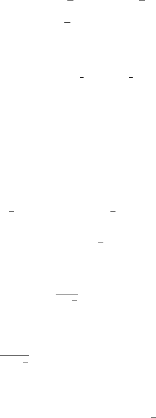
4.3. APPROXIMATION ALGORITHMS 45
X
j∈H
w(S
j
, T
j
) ≤
X
all j
K
2w(P (S
0
j
))
ν
a(S
j
)
1−ν
≤ K
2
X
all j
w(P (S
0
j
))
ν
X
j
a(S
j
)
1−ν
≤ K
2 log
n
a(V )
ν
2 log
n
a(V )
1−ν
≤ 2K
ν
log
n
a(V ) (4.3)
Here we used H¨older’s inequality: for real sequences a
1
, . . . , a
n
and b
1
, . . . , b
n
,
and any p, q ≥ 1 with (1/p) + (1/q) = 1, we have
n
X
i=1
a
i
b
i
≤
n
X
i=1
a
p
i
!
1
p
n
X
i=1
b
q
i
!
1
q
.
Next we deal with the group of cuts with low conductance within clusters
i.e., those j not in H. First, suppose that all the cuts together induce a partition
of C
i
into P
i
1
, P
i
2
, . . . P
i
r
i
. Every edge between two vertices in C
i
which belong to
different sets of the partition must be cut by some cut (S
j
, T
j
) and, conversely,
every edge of every cut (S
j
∩C
i
, T
j
∩C
i
) must have its two end points in different
sets of the partition. So, given that C
i
has conductance α, we obtain
X
all j
w
I
(S
j
∩ C
i
, T
j
∩ C
i
) =
1
2
r
i
X
s=1
w(P
i
s
, C
i
\ P
i
s
) ≥
1
2
α
X
s
min(a(P
i
s
), a(C
i
\ P
i
s
))
For each vertex u ∈ C
i
there can be at most log
n
values of j such that u belongs
to the smaller (according to a(·)) of the two sets S
j
∩ C
i
and T
j
∩ C
i
. So, we
have that
r
i
X
s=1
min(a(P
i
s
), a(C
i
\ P
i
s
)) ≥
1
log
n
X
j
min(a(S
j
∩ C
i
), a(T
j
∩ C
i
))
Thus,
X
all j
w
I
(S
j
, T
j
) ≥
α
2 log
n
l
X
i=1
X
j
min(a(S
j
∩ C
i
), a(T
j
∩ C
i
))
Therefore, from the definition of H, we have
X
j /∈H
w
I
(S
j
, T
j
) ≤ 2α
∗
X
all j
l
X
i=1
min(a(S
j
∩ C
i
), a(T
j
∩ C
i
)) ≤
2
3
X
all j
w
I
(S
j
, T
j
)
Thus, we are able to bound the intra-cluster cost of the low conductance group of
cuts in terms of the intra-cluster cost of the high conductance group. Applying
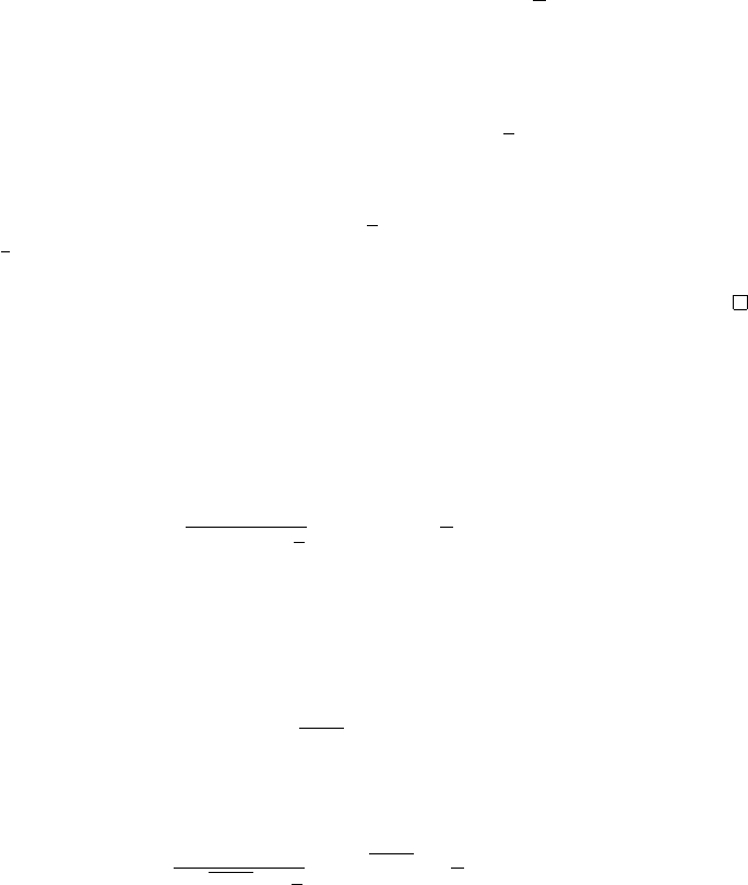
46 CHAPTER 4. RECURSIVE SPECTRAL CLUSTERING
(4.3) then gives
X
j /∈H
w
I
(S
j
, T
j
) ≤ 2
X
j∈H
w
I
(S
j
, T
j
) ≤ 4K
ν
log
n
a(V ) (4.4)
In addition, since each inter-cluster edge belongs to at most one cut S
j
, T
j
, we
have that
X
j /∈H
(w(S
j
, T
j
) − w
I
(S
j
, T
j
)) ≤
2
a(V ) (4.5)
We then sum up (4.3), (4.4) and (4.5). To get the total cost we note that
splitting up all the V
t
with a(V
t
) ≤
n
a(V ) into singletons costs us at most
2
a(V ) on the whole. Substituting a(V ) as twice the total sum of edge weights
gives the bound on the cost of inter-cluster edge weights. This completes the
proof of Theorem 4.3.
The Leighton-Rao algorithm for approximating the conductance finds a cut
of conductance at most 2 log n times the minimum [LR99]. In our terminology,
it is an approximation algorithm with K = 2 log n and ν = 1. Applying theorem
4.3 leads to the following guarantee.
Corollary 4.4. If the input has an (α, )-clustering, then, using the Leighton-
Rao method for approximating cuts, the recursive-cluster algorithm finds an
α
12 log n log
n
, 26 log n log
n
-clustering.
We now assess the running time of the algorithm using this heuristic. The
fastest implementation for this heuristic runs in
˜
O(n
2
) time (where the
˜
O nota-
tion suppresses factors of log n). Since the algorithm makes less than n cuts, the
total running time is
˜
O(n
3
). This might be slow for some real-world applica-
tions. We discuss a potentially more practical algorithm in the next section. We
conclude this section with the guarantee obtained using Arora et al.’s improved
approximation [ARV04] of O(
√
log n).
Corollary 4.5. If the input to the recursive-cluster algorithm has an (α, )-
clustering, then using the ARV method for approximating cuts, the algorithm
finds an
α
C
√
log n log
n
, C
p
log n log
n
-clustering.
where C is a fixed constant.
4.4 Worst-case guarantees for spectral cluster-
ing
In this section, we describe and analyze a recursive variant of the spectral algo-
rithm. This algorithm, outlined below, has been used in computer vision, med-
ical informatics, web search, spam detection etc.. We note that the algorithm
