Kang S.B., Quan L. Image-Based Modeling of Plants and Trees
Подождите немного. Документ загружается.


5.2. IMAGE PLANE SKETCHING 51
by Li et al. (2004) for image segmentation. For simplicity, we always use one stroke to mark the
crown. The foliage region is automatically extracted by the method described in the following
paragraph according to this stroke. The user then draws strokes to mark out branches. After each
branch stroke, a tracing algorithm is triggered to follow the visible branches close to the stroke. The
traced visible branches are displayed over the image. If not satisfied with this result, the user has
the option of adding or deleting strokes for correction. Unlike a pure sketching system (Okabe et al.
(2005)), we have the image information underlying the drawn strokes that allows extremely simple
sketching.
Figure 5.1 shows an example in which we need only two strokes: the first crown stroke in red
and the second branch stroke in blue.
Foliage extraction. Foliage is extracted from the closed region by the first crown stroke, which
roughly follows the crown boundary. ‘GrabCut’ (Rother et al. (2004)) extracts an object inside a
bounding rectangle by analyzing the different appearance inside and outside of the rectangle. The
‘GrabCut’ approach is less effective here as both inside and outside of the crown stroke could contain
a significant number of leaf colors. For extraction, we simply compute a Gaussian mixture model
(GMM) for the pixel RGB values in the region closed by the crown stroke. We employ a mixture of
10 Gaussians for large variation of colors due to the background. Then we take the four most green
or red Gaussian components as leaf clusters, and the remaining six components are considered as
background clusters. With these appearance models G(I
x
,θ
F
), G(I
x
,θ
B
) for the foreground and
background, we compute a graph-cut based extraction to detect leaf pixels. Here, G(·,θ)is the pdf
function of the GMM distribution, I
x
indicates the RGB values at pixel x, θ
F
, and θ
B
are GMM
parameters.
At each pixel x, we compute a 0 − 1 label β
x
via graph cut, where β
x
= 0 represents leaf pixels
and β
x
= 1 represents background pixels. A Gibbs energy of the following form is defined over the
enclosed region of crown stroke
x
E
d
(β
x
,θ
F
,θ
B
) +
(x,y)∈N
E
s
(β
x
,β
y
),
where N is the set of all 4-neighbor pixel pairs,
E
d
(β
x
,θ
F
,θ
B
) =−β
x
logG(I
x
,θ
B
) − (1 − β
x
)logG(I
x
,θ
F
)
is the data term, and
E
s
(β
x
,β
y
) =
0 β
x
= β
y
λ/|I
x
− I
y
| β
x
= β
y
is the smoothness term. A graph-cut algorithm (Kolmogorov and Zabih (2002)) is applied to min-
imize this Gibbs energy by assigninga0or1foreachβ
x
. The constant λ, indicating the strength
of smoothness, is set to 60 in our implementation. Before the extraction, we usually expand the
enclosed region by morphology operations to allow more freedom for the sketching by the user.

52 CHAPTER 5. SINGLE IMAGE TREE MODELING
Figure 5.2: The extracted foliage region via minimizing the Gibbs energy. These are the results for the
cherry tree in Figure 5.1 and the oak tree in Figure 5.7. Note that our modeling needs only a coarse
segmentation.
Figure 5.2 shows the result of the foliage extraction from the input image and the stroke in
Figure 5.1. Note that one important advantage of our system is that it does not require very accurate
segmentation.
Visible branch tracing. To reduce the required amount of user interaction, the system automat-
ically traces along branch strokes to detect nearby visible branches in the image. This tracing is
trigged after each branch stroke is drawn. We apply a method inspired by the ‘Lazy Snapping’
method (Li et al. (2004)). Pixels on the branch stroke are used as samples to compute an appearance
model for the branch. All the other pixels are samples to compute the non-branch appearance.Again,
a GMM model is used for the appearance model. Since the branch stroke could cover leaf pixels
(e.g., in the first example in Figure 5.7), we discard the Gaussian component in the branch GMM
if it is too close to some component in the foliage GMM G(I
x
,θ
F
). The branch appearance model
is denoted as G(I
x
,θ
T
). The appearance model for non-branch pixels is G(I
x
,θ
N
). Typically, 5
Gaussian distributions are used for each model.
With these two appearance models, we move a circle along the branch stroke from bottom
to top. At each position, pixels on the circle are classified as branch pixel or non-branch pixel by a
maximum likelihood estimation. We use a 0 −1 variable α to facilitate this classification where 0
means branch pixel and 1 for others. For each pixel x on the circle, we compute α
x
by maximizing
the following likelihood
(1 − α
x
)G(I
x
,θ
T
) + α
x
G(I
x
,θ
N
).
Typically, multiple branch pixels will be detected on the circle, with these pixels forming different
clusters. We discard a cluster if there are non-branch pixels along the line segment connecting the
cluster center and circle center (via the maximum likelihood estimation).The circle center will move
to the remaining cluster center to continue tracing. In the case of multiple clusters left on the circle,
they are processed in a breadth-first manner. The branch skeleton is detected by connecting all these
circle centers during tracing. This skeleton is overlayed in the image. If the user is not satisfied with

5.3. TREE GROWING 53
(a) (b) (c)
Figure 5.3: (a) We move a circle along the branch stroke to trace visible branches. The fork is detected
and a new green branch is created automatically. (b) The branch is recovered by connecting all circle
centers during tracing. (c) The initial branch is simplified to discard redundant joints.
this result, he or she can add more strokes to correct it or delete wrong branches.The skeleton is then
simplified by preserving the updated skeleton topology while discarding redundant joints. A joint is
deemed to be redundant if it is not located at a fork and the branch direction does not significantly
change at that joint (more specifically, if the angular change between the segments immediately
before and after the joint is less than 30
◦
). In our implementation, the circle radius is fixed at 50
pixels in all our examples, with the image resolution being about 1500 × 1500.
At the tree root, the branch thickness is also computed by varying the circle radius to find
the largest circle whose pixels are all branch pixels. This thickness computation is unreliable at small
twigs. We simply set branch radius to 75% of its parent although better botanical rules can be used
according to Weber and Penn (1995).
As shown in Figure 5.3(a), the branch segment indicated by the green line is correctly detected
although the drawn stroke does not pass through it. A branch system is retrieved by connecting circle
centers in sequence as shown in (b). This initial result contains many fragment line segments, which
is undesirable for the non-parametric synthesis in Section 5.3.1. The final branch (after redundant
joints were discarded) is shown in (c).
5.3 TREE GROWING
Once branches have been recovered, leaves can be generated along them to complete the tree. Many
previous tree modeling methods (such as Neubert et al. (2007); Xu et al. (2007) and including the
system described in Chapter 4) model trees this way by focusing on the modeling of branch systems.
Once visible branches and the foliage region are extracted from the image, we develop a tree
grow engine to automatically generate the whole tree branch in 3D space by following the given

54 CHAPTER 5. SINGLE IMAGE TREE MODELING
image. We only seek a plausible solution that is possible with the tree priors and the inherent self-
similar structural patterns of the tree. A production engine similar to that of Xu et al. (2007) and
the system described in Chapter 4 is used where 3D points are used to guide the growth.
5.3.1 GROWTH ENGINE
The engine starts with the creation of a library of elementary subtrees from the visible branches.
Then, a non-parametric synthesis approach is used to systematically generate branches that were
occluded in the image.
Initialization. There are two parts in the initialization process, namely conversion of 2D branches
(from the image) to 3D and generation of the subtree library.
• Conversion of 2D branches into 3D: Visible branches interactively traced in Section 5.2 are
defined in the image plane. We first convert these branches from 2D to 3D before growing.
From a single image, there is not enough information to accurately reconstruct the branch
position in 3D space. Here, we employ the approach proposed in Okabe et al. (2005) to gen-
erate a 3D branch structure from the extracted visible branches. The basic idea is to distribute
branches in 3D space evenly and keep their image projections unchanged. Here, we assume
an orthographic camera model to relate 3D branch position and image coordinate.
• Creation of the library: We then built a library of elementary subtrees. These library subtrees
are built from the recovered visible branches by taking all its subtrees. If there are too few sub-
trees (as in the first example in Figure 5.7), we add predefined subtrees in the library. Figure 5.4
shows the predefined subtrees in our implemented system. Obviously, this predefined library
can be further enriched to handle larger varieties of trees. It is remarkable that we produced
all of our results with only at most 8 subtrees in the current implementation.
Non-parametric synthesis. Starting from the 3D visible branch and a library, we take a non-
parametric approach to grow a tree. The synthesis process simply iteratively replaces an existing
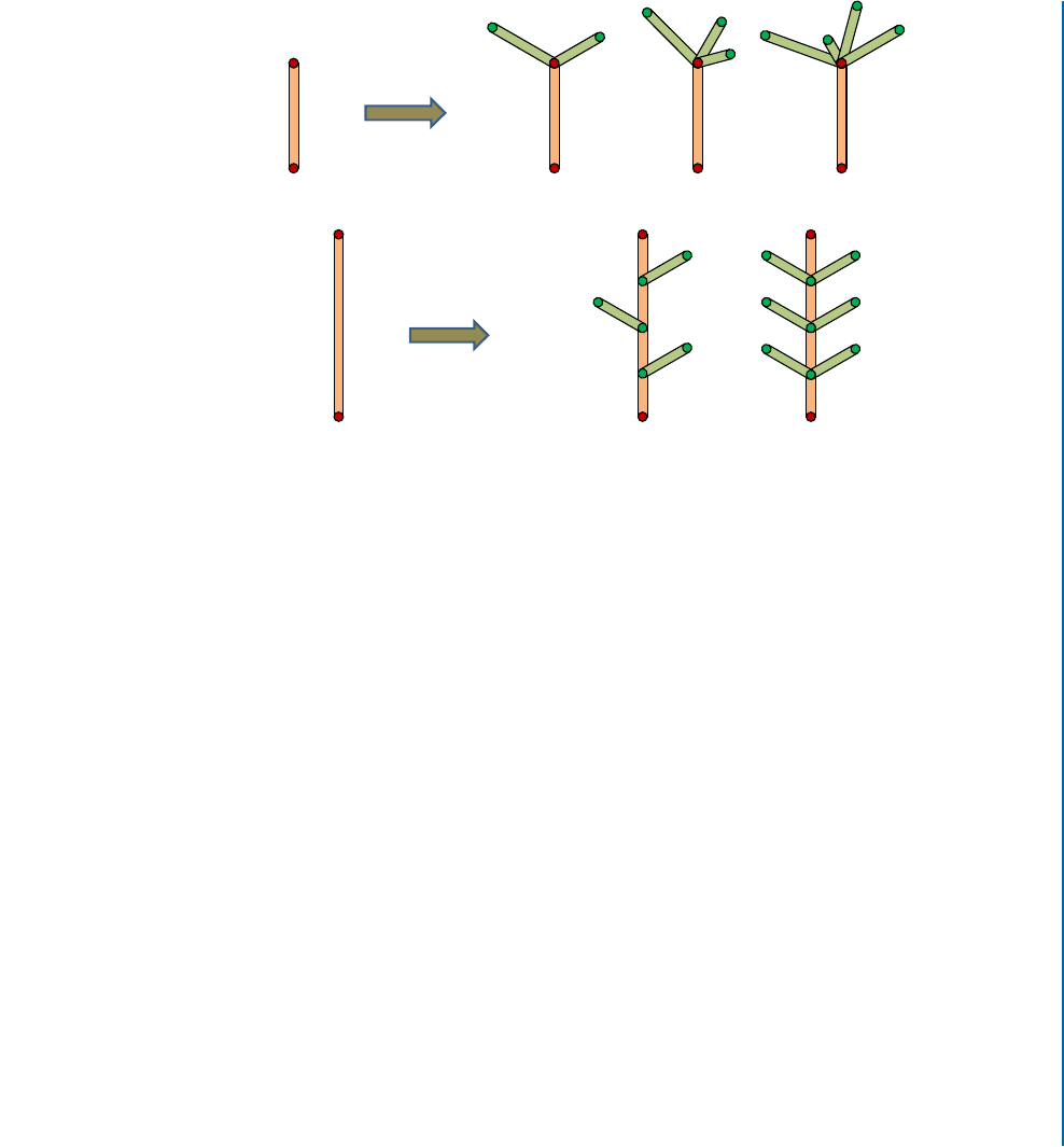
branch by a library subtree. Figure 5.4 shows a single step of the non-parametric branch growth.
There are two types of branch replacement in our system. In type I replacement, new branches
grow at the end of its ‘supporting branch’ (i.e., shown as the red segment in a subtree). In type II
replacement, new branches can grow along the ‘supporting branch.’
The selection of the branch to be replaced and the library subtree is driven by minimizing the
cost function defined in Section 5.3.2. Each time, the resulting synthesis is pruned by the extracted
foliage silhouette. Usually, we run the following three steps iteratively about 100 times for each tree:
• Selection of a branch to be replaced: We go through a small set of existing branches and take
the one whose replacement gives the lowest cost function defined in Section 5.3.2.
5.3. TREE GROWING 55
(a) Type I branch replacement
(b) Type II branch replacement
Figure 5.4: A branch is replaced by a library subtree. We call the red branch in the subtree as ‘supporting
branch’ for ease of reference.
To create this set of existing branches, we choose branches with larger radius and older gen-
eration. We sort all existing branches according to their radius. Then branches are selected
sequentially from the sorted array. Each branch is selected with a probability, which is inversely
proportional to its generation.
• Selection of a replacing library subtree: For the selected branch to be replaced, we search all
the available library subtrees (at most (8) to find that one giving the lowest cost of the function
defined in Section 5.3.2.
Except for the subtrees generated from visible branches, the user can add predefined subtrees:
type I, type II or both. A subtree is rotated around its ‘supporting branch’ and scaled before
it is used to replace some existing branch. There are two parameters to be determined in this
operation.
– The rotation angle of the subtree around its ‘supporting branch’ is searched among 12
quantized levels of 360 degrees that gives the lowest cost.
– The scaling factor of the subtree is determined such that its ‘supporting branch’ is of the
same length as the replaced branch.
• Branch pruning: After replacement, the resulting branches are pruned based on the detected
foliage region and the existing branches. Any branch going beyond the foliage region is re-
moved, as are the new branches if they are too close to some existing branches.
56 CHAPTER 5. SINGLE IMAGE TREE MODELING
(a) (b)
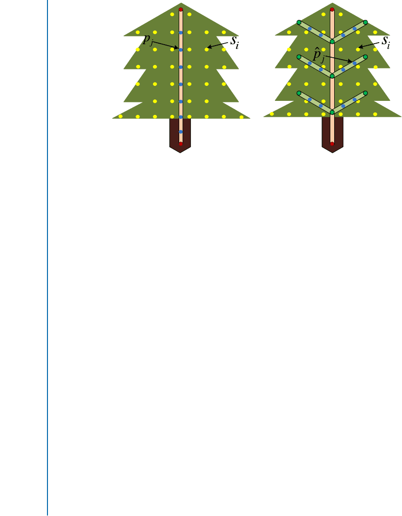
Figure 5.5: Yellow points in the foliage region are the image attractors. (a) Blue points are sampled over
the tree to compute the distance between an attractor and the tree. (b) After branch replacement, the
distance between attractors and the tree is updated according to newly created branches.
5.3.2 DATA-DRIVEN ATTRACTORS
The growth engine is driven by the data to produce a realistic result. The input image information
is 2D and only weakly controls the growth in the desired tree volume. Hence, we introduce some
3D points based on heuristics to control the growth better.
Image attractors. To make the result after growing similar to the image, we define a set of image
attractors s
i
,i ={1, 2, ···N} that are sampled evenly in the foliage region with a fixed interval as
illustrated by the yellow points in Figure 5.5 (a).These attractors control the tree growth by requiring
that each attractor should be close to the resulting tree T . The growth is then driven by minimizing
a cost defined as E
2D
(T ) =
i
dist(s
i
,T), where dist(s
i
,T) is the distance of an attractor s
i
to
the projection of tree T onto the image. To compute dist(s
i
,T), we also sample a set of points
p
i
,i ={1, 2, ···M} along the image projection of the tree T as the blue points in Figure 5.5 (a).
The distance function is then defined as dist(s
i
,T) = min
j
(dist (s
i
,p
j
)).
Extrapolated 3D attractors. The image driven growth could lead to an unbalanced tree, where
only front branches are generated. This is because such an unbalanced tree can minimize the cost
E
2D
(T ) well without any back branches. Similar problems exist in previous sketching systems such
as Okabe et al. (2005). To alleviate this problem, the tree is rotated 90 degrees around its main trunk
and merged with the original one, as in Okabe et al. (2005). This method solves the problem at the
cost of creating inconsistent visible branches with the image.

5.4. COMPLETING THE TREE 57
We introduce some extrapolated 3D points to balance the tree growth. We rotate the existing
tree by 90
◦
, but only keep its branch joints d
i
,i ={1, 2, ···K}. These joints are used as 3D space
attractors to drive branch replacement in a similar manner to image attractors. Here the distance
between these 3D points and the tree is to be minimized and the cost is defined as E
3D
(T ) =
i
dist(d
i
, T ). dist (d
i
,T) is the distance between the 3D point d
i
and the tree T . Again, the
tree T is sampled as a set of points t
i
,i ={1, 2, ···,L} in 3D space along the branch skeleton to
compute the dist(d
i
,T) = min
j
(dist (d
i
,t
j
)).
In our current implementation, the growth is driven by alternating the image attractors and
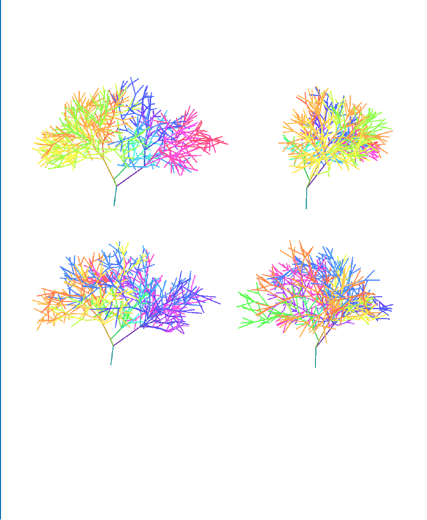
the 3D point attractors. Figure 5.6 illustrates the effectiveness of this alternating strategy. The pure
image driven growth yields good results when viewed from the same direction as the input image,
as in (a), and unnatural results (b) viewed from an orthogonal viewpoint. By alternating the image
driven growth and 3D point driven growth, a better result can be obtained in (c) and (d).
Speedup. The growth engine involves a large amount of computation of the distances between
the attractors and the tree. In each replacement iteration, we only add more branches to the tree
and no existing branch is discarded. So the distance computation in the previous iteration can be
reused for speedup purposes. For each attractor s (no matter image point or 3D point), we record
its distance to the tree T
n
at the n−th iteration as d
n
s
. At the n + 1−th iteration, we compute the
distance between s and newly created branches as
ˆ
d
s
. The distance between s and T
n+1
is then
updated as d
n+1
s
= min{d
n
s
,
ˆ
d
s
}. This is illustrated in Figure 5.5(b).
5.4 COMPLETING THE TREE
The leaves of the tree are automatically synthesized from the recovered branch structure and textured
with the input image. Each leaf is represented by a flat rectangle with the size of 1/10 of the main
trunk radius. Each branch generates from a range of 50 to 200 leaves proportional to it length.
The arrangement of the leaves around the branch is randomized. We keep only those leaves that
are projected inside the foliage region in the input image. Leaves are textured according to their
projected position on the input image. The generic leaf shape, leaf size, density and arrangement of
leaves along a branch are all parameterized in our current implementation. But the default values
are used throughout all examples of this chapter.
5.5 RESULTS
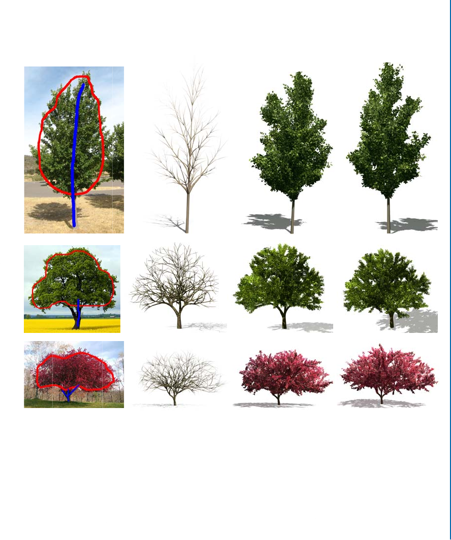
We tested our system on several different examples to demonstrate its effectiveness. One example
(image of a cherry tree downloaded from www.flickr.com) is shown in Figure 5.1. Its foliage region
is shown in Figure 5.2, and its branch tracing procedure is illustrated in Figure 5.3. The complete
branching structure generated by the growth engine is shown in Figure 5.1(c). A rendering of the
final cherry tree model is shown in Figure 5.1(d). For this example, we drew two strokes and used
both subtrees of visible branches and predefined subtrees of type I. Branch tracing was performed
58 CHAPTER 5. SINGLE IMAGE TREE MODELING
(a) (b)
(c) (d)
Figure 5.6: (a) and (b) are the branches generated by image driven growth viewed from the front and
side. Although the image driven growth can guarantee the result similar to the image in front, the result
looks unnatural from the side. (c) and (d) are results computed by alternating image driven growth and
3D point driven growth. Both front and side results look good.
5.5. RESULTS 59
(a) (b) (c) (d)
Figure 5.7: Examples are sorted by increasing number of strokes: (a) The single input image. (b) The
synthesized branch structure. (c) Complete tree model with leaves rendered at the same viewpoint as the
input image. (d) Rendered from a novel view point.
60 CHAPTER 5. SINGLE IMAGE TREE MODELING
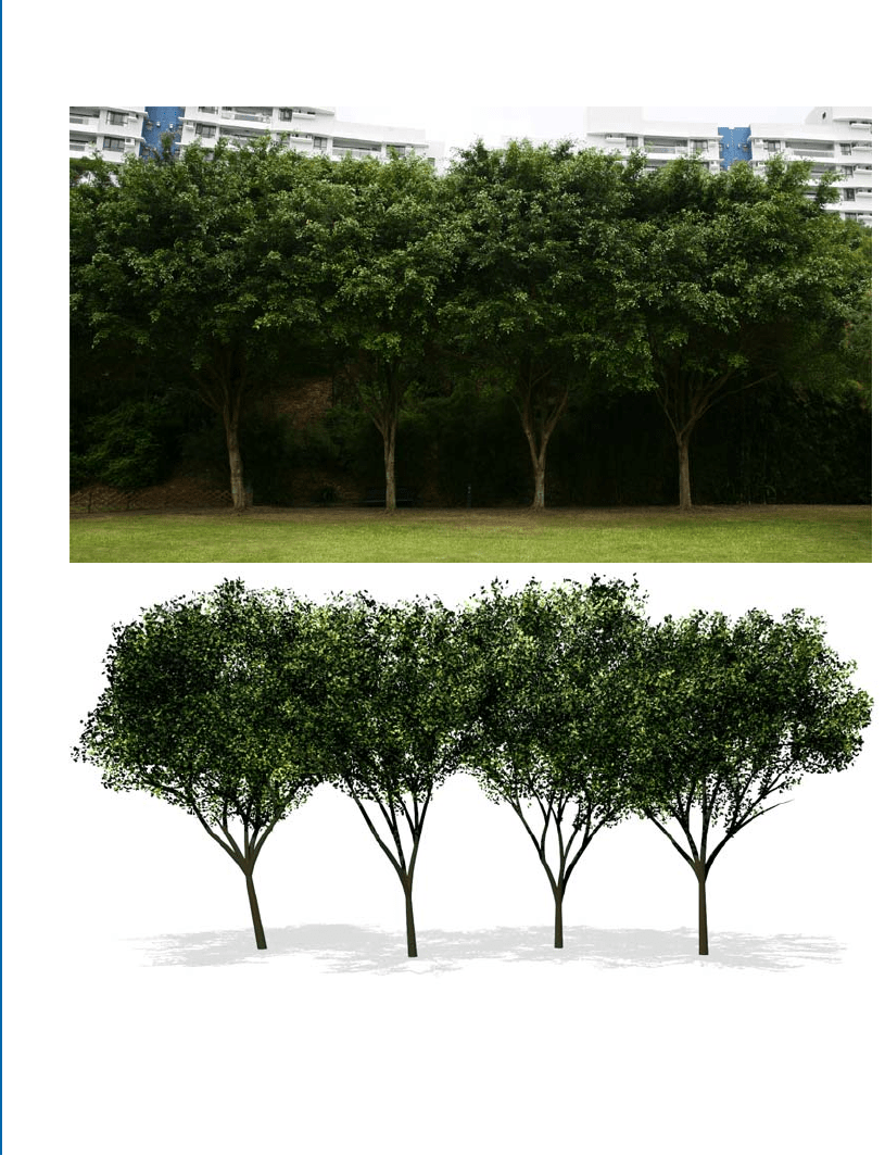
Figure 5.8: Modeling woods with multiple trees. On the top is the input image. The rendering of the
recovered model is at the bottom.
