Jaeger G. Quantum Information: An Overview
Подождите немного. Документ загружается.


6
Quantum entanglement
Quantum interference arises from the indistinguishability in principle, by pre-
cise measurement at a specified final time, of alternative sequences of states
of a quantum system that begin with a given initial state and end with the
corresponding final state. It is manifested, for example, in the two-slit inter-
ferometer and the double Mach–Zehnder interferometer discussed in Chapters
1 and 3, respectively. Most important, when the indistinguishability of alter-
natives for producing joint events arises, as in the latter apparatus, entangle-
ment may be involved. Erwin Schr¨odinger, who first used the term “entangle-
ment,” called entanglement “the characteristic trait of quantum mechanics”
[364, 365, 366]. The extraordinary correlation between quantum subsystem
states associated with entanglement can be exploited by quantum computing
algorithms using interference to solve computational tasks, such as factoring,
far more efficiently than is possible using classical methods, as we show in
later chapters. Entangled states are similarly exploitable by uniquely quantum
communication protocols, such as quantum teleportation, superdense coding,
and advanced forms of quantum key distribution, using local operations and
classical communication (LOCC).
Entanglement is of perennial intrinsic interest because of the radically
counter-intuitive behavior associated with the strong correlations it entails,
that was discussed in Chapter 3. Albert Einstein, Boris Podolsky, and Nathan
Rosen argued early on that quantum mechanics is incomplete if understood as
a local realistic theory, based on the consideration of an (entangled) quantum
state of the form
|Ψ(x
1
,x
2
) =
∞
i=1
a
i
|ψ(x
1
)
i
|φ(x
2
)
i
(6.1)
[147]. David Bohm later explored entanglement in a far simpler context, that
of a pair of spins in the singlet state
|Ψ
−
=
1
√
2
(| ↑↓ − | ↓↑) , (6.2)

92 6 Quantum entanglement
which has since been central to the investigation of the foundations of quantum
mechanics and quantum information, wherein {| ↑, | ↓} is typically taken as
the computational basis and written {|0, |1} [66].
Following these developments, John Bell greatly advanced the investiga-
tion of quantum entanglement by clearly delimiting the border between local
classically explicable behavior and less intuitive sorts of behavior that are non-
local, by deriving an inequality that must be obeyed by local realistic theories
that might explain strong correlations between two distant subsystems form-
ing a compound system, such as those arising in systems described in quantum
mechanics by the singlet state [30]. Since these early investigations, the study
of extraordinarily correlated behavior between subsystems within larger sys-
tems has been ongoing, as have efforts to put this unusual behavior to use.
In this chapter, we consider the current understanding of quantum entangle-
ment in bipartite quantum systems, which often uses the various quantum
information measures introduced in the previous chapter.
6.1 Basic definitions
Under Schr¨odinger’s definition, entangled pure states are simply those pure
quantum states of multipartite systems that cannot be represented in the form
of a simple tensor product of subsystem states
|Ψ = |ψ
1
⊗|ψ
2
⊗···⊗|ψ
n
, (6.3)
where |ψ
i
are states of local subsystems, for example, spin states of funda-
mental particles [365, 366]. The remaining pure states of multipartite systems,
which can be represented as simple tensor products of independent subsystem
states, are called simply product states. The definition of entanglement can
be extended to include mixed states, as follows. The mixed quantum states
in which entanglement is most easily understood are states ρ
AB
of bipartite
systems, usually labeled AB with components labeled A and B in correspon-
dence with the laboratories where they are located. Mixed states are called
separable (or factorable) when they can be written as convex combinations
of products,
ρ
AB
=
i
p
i
ρ
Ai
⊗ ρ
Bi
, (6.4)
where p
i
∈ [0, 1] and
i
p
i
=1,ρ
A
and ρ
B
being statistical operators on
subsystem Hilbert spaces, H
A
and H
B
, respectively.
1
Entangled quantum
states are simply those that are inseparable.
Separable mixed states contain no entanglement, as they are by defini-
tion the mixtures of product states and so can be created by local operations
1
This definition extends beyond the statistical operators to other operators, gen-
eralizing the concept of entanglement beyond states.

6.1 Basic definitions 93
and classical communication from pure product states: in order to create a
separable state, an agent in one lab needs merely to sample the probability
distribution {p
i
} and share the corresponding measurement results with an
agent the another; the two agents can then create their own sets of suitable
local states ρ
i
in their separate labs.
2
However, by contrast, not all entangled
states can be converted into each other in this way in the multi-party context,
something that leads to distinct classes of entangled states and thus to differ-
ent sorts of entanglement, as we show in the next chapter. In general, it is also
not always possible to tell whether a given statistical operator is entangled.
Given a set of subsystems, the problem of determining whether their joint
state is entangled is known as the separability problem.
The simplest states within the class of separable states are the product
states of the form ρ
AB
= ρ
A
⊗ρ
B
; ρ
A
and ρ
B
are then also the reduced statis-
tical operators for the two subsystems and are uncorrelated. When there are
correlations between properties of subsystems described by separable states,
these can be fully accounted for locally because the separate quantum states
ρ
A
and ρ
B
within spacelike-separated laboratories provide descriptions suffi-
cient for common cause explanations of the joint properties of A and B such
as that outlined above; also see [430]. In particular, the outcomes of local mea-
surements on any separable statistical operator can be simulated by a local
hidden-variables theory. The quantum states in which correlations between A
and B can be seen to violate a Bell-type inequality, referred to as Bell corre-
lated (or EPR correlated) states, cannot be accounted for by common cause
explanations. If a pure state is entangled then it is Bell correlated.
3
Thus,
pure entangled states do not admit a common cause explanation. However,
this is not true for the mixed entangled states. For example, the Werner state,
ρ
W
=
1 −
1
√
2
1
4
I ⊗ I +
1
√
2
P (|Ψ
−
) , (6.5)
is not Bell correlated yet is entangled, because there is no way to write ρ
W
as a convex combination of product states; in particular, it cannot be written
in the form of Eq. 6.4 with only one nonzero p
i
.
4
The shortcoming of Bell-inequality violation as a necessary condition for
entanglement is that it is unknown whether there exist Bell inequality viola-
tions for many nonseparable mixed states. In the presence of manipulations
of such a state (or a collection of copies) by means of LOCC, some states can
be made to violate a Bell-type inequality; those states that can be made to
2
See Chapter 3 for a characterization of local operations.
3
This was first pointed out by Sandu Popescu and Daniel Rohrlich [338] and
Nicolas Gisin [186]. Note, however, that not all such states are Bell states, that
is, elements of the Bell basis as, say, |Ψ
−
is; see Sect. 6.3, below [339].
4
Note also that the Werner state is diagonal in the Bell-basis representation. An
excellent review discussing the relationship between Bell inequalities and entan-
glement is [451].

94 6 Quantum entanglement
violate a Bell inequality in this way are referred to as distillable states. The
remaining, nondistillable states are known as bound states. What is clear is
that state entanglement should not change under local operations and should
not be increased by local operations together with classical communication,
assumptions that play a central role in quantifying entanglement, as we show
in Section 6.6 below. Let us first consider some fundamental tools in the study
of entanglement.
6.2 The Schmidt decomposition
There exist special state decompositions that clearly manifest the correlations
associated with entanglement. For pure bipartite states, the Schmidt decom-
position serves this purpose well. Any bipartite pure state |Ψ ∈H= H
A
⊗H
B
can be written as a sum of bi-orthogonal terms: there exists at least one or-
thonormal basis for H, {|u
i
⊗|v
i
} where {|u
i
} ∈ H
A
and {|v
i
} ∈ H
B
such
that
|Ψ =
i
a
i
|u
i
⊗|v
i
, (6.6)
a
i
∈ C, referred to as a Schmidt basis. This representation is a Schmidt (or
polar) decomposition of |Ψ, where the summation index runs up only to
the smaller of the corresponding two Hilbert space dimensions, dim H
A
and
dim H
B
[363]. It is often convenient to take the amplitudes a
i
to be real
numbers by absorbing any phases into the definitions of the {|u
i
} and {|v
i
}.
Unfortunately, the availability of this decomposition in multipartite systems
is limited, being available with certainty only in the case of bipartite states.
For any entangled bipartite pure state, it is possible to find pairs
of measurable quantities violating the Bell inequality. In particular,
the Schmidt observables
U =
i
u
i
|u
i
u
i
| , (6.7)
V =
i
v
i
|v
i
v
i
| , (6.8)
are fully correlated when the system is in state |Ψ, providing such
violations [186].
The number of nonzero amplitudes a
i
in the Schmidt decomposition of a
quantum state is known as the Schmidt number (or Schmidt rank), Sch(|Ψ).
The Schmidt number proves useful for distinguishing entangled states. In par-
ticular, the Schmidt number of a state is greater than 1 if and only if it is
entangled. It is useful as a (coarse) quantifier of the amount of entanglement
in a system, in addition to serving as a criterion for entanglement.

6.3 Special bases and decompositions 95
The Schmidt number of a bipartite system is equivalently defined as
Sch(|Ψ) ≡ dim supp ρ
A
= dim supp ρ
B
, (6.9)
where ρ
A
and ρ
B
are the reduced statistical operators for the two subsystems,
ρ
A
=
i
|a
i
|
2
|u
i
u
i
| , (6.10)
ρ
B
=
i
|a
i
|
2
|v
i
v
i
| , (6.11)
which are diagonal, possess identical eigenvalue spectra, and hence have identi-
cal von Neumann entropies. Furthermore, Schmidt number is preserved under
local unitary state transformations.
Using the Schmidt decomposition, the Schmidt measure (Hartley strength)
oftheentanglementofpurestatesisdefinedas
E
S
(|Ψ) ≡ log
2
Sch(|Ψ)
, (6.12)
providing entanglement in units of “e-bits,” a term, like “qubit,” introduced
by Schumacher, where the Bell states correspond to one e-bit of entangle-
ment. The probabilities that are the squares of the Schmidt coefficients a
i
are precisely those quantities unchanged by unitary operations performed lo-
cally on the individual subsystems (LUT’s). For this reason, it is reasonable
to expect any more precise numerical measure of pure state entanglement to
be calculable from the quantities |a
i
|
2
.
5
Because the statistical operator ρ of
a bipartite system may have degenerate eigenvalues there is, however, not a
truly unique Schmidt basis. For example, in the case of the Bell state |Ψ
−
,
the state takes the same form when represented in any other basis obtained
from the computational basis representation (Eq. 3.5), which is of Schmidt
form, by rotating the computational basis and performing a unitary transfor-
mation in the subspace of the first qubit and the conjugate transformation in
that of the second qubit [154].
Again, the Schmidt decomposition is not always available beyond the case
of bipartite systems. Consider the case of a system with three subsystems. If
there existed such a decomposition, the measurement of one subsystem would
provide the states of the remaining two; but, if these two are entangled, then
the individual states must be indefinite.
6
6.3 Special bases and decompositions
BasicexamplesofstatesinSchmidtformarethefourelementsoftheBell
basis, which are the entangled states written
5
One example of this is the concurrence, defined in Sect. 6.10, below.
6
The generalization of this decomposition to special states of larger systems where
such a decomposition does exist, such as the GHZ state |GHZ =(1/
√
2)(|000+
|111), is discussed briefly later in Sect. 7.3.
96 6 Quantum entanglement
|Ψ
±
=
1
√
2
(|01±|10) (6.13)
|Φ
±
=
1
√
2
(|00±|11) (6.14)
in the computational basis and which are symmetrical or antisymmetrical
under qubit exchange. These Bell states have played a central role in the
investigation of quantum entanglement and tests of local realism, as shown
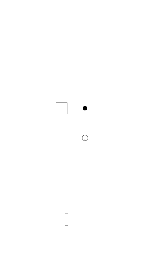
in Chapter 3. The creation of the states of the Bell basis from a pair of
unentangled qubits can be carried out by a process described by a quantum
circuit involving only one Hadamard and one C-NOT gate; see Fig. 6.1. Bell
states are also readily produced ab initio using spontaneous parametric down-
conversion, which is discussed in Section 6.16. Bell states have the useful
property that transforming the state of only one subsystem locally suffices for
interconversion between them, which is not true, for example, of the two-qubit
computational-basis states, which are of product form. Of particular interest
is the singlet state, |Ψ
−
, due to its great symmetry.
H
|b
1
Ó
|B
b
1
b
2
Ó
|b
2
Ó
Fig. 6.1. A quantum circuit for the synthesis of Bell states, |B
b
1
b
2
from a product
state. The input states are indicated by the bit values b
i
∈{0, 1},i=1, 2: b
1
b
2
=
00, 10, 01, 11 yield |Φ
+
, |Φ
−
, |Ψ
+
, |Ψ
−
, respectively.
Another basis of entangled states for two-qubits, the so-called “magic
basis,” is similar to the Bell basis but has different overall phases and
norm,
|m
1
=
1
2
(|00 + |11) , (6.15)
|m
2
=
i
2
(|00−|11) , (6.16)
|m
3
=
i
2
(|01 + |10) , (6.17)
|m
4
=
1
2
(|01−|10) , (6.18)
and is a natural one for concurrence-based entanglement studies,
discussed in Section 6.10, below [214].

6.3 Special bases and decompositions 97
Another useful basis is the q-basis,
|q
1
=
√
q|00+
1 − q|11 , (6.19)
|q
2
=
1 − q|00−
√
q|11 , (6.20)
|q
3
=
√
q|01+
1 − q|10 , (6.21)
|q
4
=
1 − q|01−
√
q|10 , (6.22)
which, for values q ∈ [0, 1], interpolates between the (product) com-
putational basis (for which q =0, 1) and the (entangled) Bell basis
(for which q =1/2). Varying the value of q, say by taking q =cosθ
and varying θ, allows one to study the role of entanglement over this
important range of pure states; for example, see Section 9.11 and
[234].
A Lewenstein-Sanpera (LS) decomposition of a statistical operator ρ ∈
C
2
⊗ C
2
is one of the form
ρ = λρ
sep
+(1− λ)P (|Ψ
ent
) , (6.23)
with λ ∈ [0, 1], where ρ
sep
is separable and P (|Ψ
ent
) is the projector for
a fully entangled state [282]. Such a decomposition exists for any two-qubit
state. Although this decomposition is not unique, the decomposition for which
λ takes an optimal value, λ
max
, is. λ
max
is sometimes referred to as the degree
of separability and can be viewed as the degree of classicality of the state.
7
One example following from the LS decomposition is the Werner state (cf.
Equation 6.5, above). Varying λ allows one to explore the role of entanglement
over an important range of mixed states; for example, see [309].
Yet another useful class of basis is that of the unextendable product bases,
which are sets of orthogonal product state-vectors such that there exists no
additional product state-vector orthogonal to them in order to span the entire
space in which they lie [45, 203]. A two-qutrit example is
|υ
1
=
1
√
2
|0(|0−|1) , (6.24)
|υ
2
=
1
√
2
(|0−|1)|2 , (6.25)
|υ
3
=
1
√
2
(|1−|2)|0 , (6.26)
|υ
4
=
1
√
2
|2(|1−|2) , (6.27)
|υ
5
=
1
3
(|0 + |1+ |2)(|0+ |1+ |2) . (6.28)
7
Such a decomposition, which was anticipated by Shimony (see Sect. 6.15 and
[383]), is known as the best separable approximation.

98 6 Quantum entanglement
6.4 Stokes parameters and entanglement
As we saw in Chapter 1, qubits have a variety of representations, among these
the real-valued one provided by the single-qubit Stokes parameters. Although
they suffice when specifying individual qubits or several qubits in a separable
state, the single-qubit parameters must be supplemented by additional pa-
rameters in order to describe entangled systems. Consider the general state
of a pair of qubits. The two-particle Stokes parameters, S
µν
≡ tr(ρσ
µ
⊗ σ
ν
)
(µ, ν =0, 1, 2, 3), which are a generalization of the traditional Stokes param-
eters, are needed to describe entangled states, such as the Bell states, in the
real representation, due to the increasing complexity of quantum states as
number of qubits grows.
8
The two-qubit Stokes parameters, introduced by
Ugo Fano just before 1950, can also be used to find the two-qubit statistical
operator:
ρ =
1
4
3
µ,ν=0
S
µν
σ
µ
⊗ σ
ν
, (6.29)
where σ
µ
⊗ σ
ν
(µ, ν =0, 1, 2, 3) are tensor products of the identity and Pauli
matrices [166];
9
the single-qubit Stokes parameters are recovered when either
µ or ν is zero, so that the corresponding factor is an identity matrix.
The Stokes four-vector [S
µ
] described in Section 1.3 is similarly general-
ized, as one can view the two-qubit Stokes parameters as forming a 16-element
Stokes tensor,[S
µν
].
10
This tensor captures all the quantum correlations po-
tentially present in a two-qubit system and plays a central role in the quan-
tum state tomography of such a system, corresponding to a compendium of
coincidence-measurement data.
11
For example, the Bell state |Ψ
+
corresponds
to a Stokes tensor with S
00
=1,S
11
= −1,S
22
= −1,S
33
= 1, the remaining
parameters being zero. The Lorentz group invariant for the two-qubit Stokes
tensor,
S
2
(2)
P (|ψ)
=
1
4
(S
00
)
2
−
3
i=1
(S
i0
)
2
−
3
j=1
(S
0j
)
2
+
3
i=1
3
j=1
(S
ij
)
2
, (6.30)
can be related to the entanglement of the two-qubit state, as we show in
Section 7.4 [237].
8
The practical value of the generalized Stokes parameters is manifest in their
application to polarization-entangled photon pairs; for example, see [3].
9
Recall that the Hilbert space for two-qubit systems is C
2
⊗ C
2
. The two-qubit
density matrices ρ are positive, unit-trace elements of the 16-dimensional complex
vector space of Hermitian 4 ×4 matrices, H(4). The operators σ
µν
≡ σ
µ
⊗σ
ν
pro-
vide a basis for H(4), which is isomorphic to the tensor product space H(2)⊗H(2)
of the same dimension, because
1
4
tr(σ
µν
σ
αβ
)=δ
µα
δ
νβ
and σ
2
µν
= I
2
.
10
The term “Stokes tensor” was first applied to this structure in [240].
11
Quantum state tomography is discussed in Chapter 8.

6.5 Partial transpose and reduction criteria 99
The elements of the general two-particle matrix ρ =
ρ
µν
are re-
lated to the two-qubit Stokes tensor elements S
µν
by the following
relations.
S
00
= ρ
00
+ ρ
11
+ ρ
22
+ ρ
33
(6.31)
S
01
= 2Re(ρ
01
+ ρ
23
) (6.32)
S
02
= −2Im(ρ
01
+ ρ
23
) (6.33)
S
03
= ρ
00
− ρ
11
+ ρ
22
− ρ
33
(6.34)
S
10
= 2Re(ρ
02
+ ρ
13
) (6.35)
S
11
= 2Re(ρ
03
+ ρ
12
) (6.36)
S
12
= −2Im(ρ
03
− ρ
12
) (6.37)
S
13
= 2Re(ρ
02
− ρ
13
) (6.38)
S
20
= −2Im(ρ
02
+ ρ
13
) (6.39)
S
21
= −2Im(ρ
03
+ ρ
12
) (6.40)
S
22
= −2Re(ρ
03
− ρ
12
) (6.41)
S
23
= −2Im(ρ
02
− ρ
13
) (6.42)
S
30
= ρ
00
+ ρ
11
− ρ
22
− ρ
33
(6.43)
S
31
= 2Re(ρ
01
− ρ
23
) (6.44)
S
32
= −2Im(ρ
01
− ρ
23
) (6.45)
S
33
= ρ
00
− ρ
11
− ρ
22
+ ρ
33
. (6.46)
6.5 Partial transpose and reduction criteria
In addition to the Schmidt number, Sch(|Ψ), and Schmidt measure, E
S
,for
pure states described in Section 6.2 above, another simple quantity measuring
entanglement for some mixed states is the negativity, N(ρ). This quantity
involves the sum of the negative eigenvalues of the partial transpose of the
density matrix of a bipartite system. It was first used to provide a criterion for
entanglement by Asher Peres, who noted that when the partial transposition
operation is performed on a separable mixed state the result is always another
mixed state [329]. Partial transposition is matrix transposition relative to the
indices of a subsystem; the matrix elements of the partially transposed density
matrix are thus
i
A
j
B
|ρ
T
A
|k
A
l
B
≡k
A
j
B
|ρ|i
A
l
B
. (6.47)
Specifically, the “Peres–Horodeˇcki (PH) criterion” for entanglement is the
following: a state ρ is entangled if the partial transpose of the corresponding
density matrix is negative. One can take
N(ρ)=
1
2
||ρ
T
A
||
1
− 1
, (6.48)

100 6 Quantum entanglement
where ||ρ
T
A
||
1
is the trace-norm of the partial transpose matrix. Because
||O||
1
≡ tr
√
O
†
O for any Hermitian operator O,onecanwrite
N(ρ)=
i
λ
i
, (6.49)
where i runs over the negative values among the set of eigenvalues {λ
i
(ρ
T
B
)}
of this density matrix.
12
The negativity is readily computed and has been used to develop entan-
glement bounds. Its logarithm, the logarithmic negativity, is also sometimes
considered, because it has operational interpretations such as an upper bound
to the distillable entanglement considered, a bound on teleportation capacity,
and an asymptotic entanglement cost under PPT; see Section 6.8 below and
[17, 42].
The positivity of ρ
T
A
(or ρ
T
B
) is a necessary and sufficient condition
for the separability of the statistical operator ρ for 2×2, 2×3dimen-
sional systems and for two continuous-variable systems (modes) in a
Gaussian state [141]. For a related result not making use of a map
between matrices that is linear, as partial transposition is, but rather
a nonlinear map to solve the separability problem for Gaussian states
of an arbitrary number of modes per site, see [181].
When applied to a Bell state, the result of partial transposition is a
matrix with at least one negative eigenvalue. Positivity of the par-
tial transpose is, in general, a necessary but insufficient condition for
separability when subsystems with Hilbert spaces of higher dimen-
sion than that of a qubit are involved; for larger Hilbert spaces, there
exist entangled states whose density matrices are positive under par-
tial transpose (PPT). See Section 6.11 below for further discussion
of the PH criterion and examples of states having PPT.
The “PPT preserving” class of quantum operations includes all bi-
partite quantum operations for which input states that are positive
under partial transposition have output states that also have this
property; these operations can produce only the bound variety of
entanglement; see Section 6.8, below.
For the bound entangled states with PPT, all CHSH-inequalities are
obeyed. The PH criterion implies another useful criterion, namely, both
ρ
A
⊗ I −ρ ≥ 0 , (6.50)
I ⊗ ρ
B
− ρ ≥ 0 , (6.51)
12
The eigenvalues of the density matrix are usually indicated in ascending order.