I. Ramos Arreguin (ed.) Automation and Robotics

Подождите немного. Документ загружается.

Closed-Loop Feedback Systems in

Automation and Robotics,

Adaptive and Partial Stabilization

G. R. Rokni Lamooki

Center of Excellence in Biomathematics, Faculty of mathematics statistics and Computer

Science, College of Science, University of Tehran

Iran

1. Introduction

Feedback controls have applications in various fields including engineering, mechanics,

biomathematics, and mathematical economics; see (Ogata, 1970), (de Queiroz, et al. 2000),

(Murray, 2002), and (Seierstad & Sydsaeter, 1987) for more details. Lyapunov based control

of mechanical system is a well-known technique. This includes Lyapunov direct/indirect

methods. Such techniques can be employed to control the whole state variables or a part of

the state variables. Sometimes there are some uncertainties or some reference trajectories

which requires adaptive control. Back-stepping is a yet powerful approach to design the

required controller. However, this approach leads to a complicated controller, especially

when the chain of integrators is long. Back-stepping can also be used when the aim of

control is the stability with respect to a part of the variables. These three concepts emerge in

a mechanical system like a robot. Adaptive control can be carried out through two different

approaches: indirect and direct adaptive control. Nevertheless there are some drawbacks in

such control systems which are a matter of concern. For example, when there is the

possibility of fault or it is considered to turn off the adaptation for saving energy, when the

system seems to be relaxed at its equilibrium situation, the outcome can be dramatically

destructive. Adaptively controlled systems with unknown parameters exhibit partial

stability phenomenon when the persistence of excitation is not assumed to be satisfied by

the designed controllers. Partial stability technique is most useful when a fully stabilized

system losses some control engine or some phase variables are not actively controlled. Such

situation is most applicable for automatic systems which need to work remotely without a

proper access to maintenance; e.g., satellite, robots to work on other planets or under hard

conditions which are required to continue their mission even if some fault happens, or when

a minimum of controller is required. It is also applicable to biped robots when one of the

engines is turned off, or weakened, for lack of energy or fault or when the robot is passively

designed. It is worth noting that another useful aspect of partial stability and control is the

possibility of controlling the required part of the phase variables without spending energy

to control the part of the variables which is not relevant to the mission of the designed

system. These concepts will be explained through some examples. The results will be

illustrated by numerical computations. This chapter is organized as follows. In section 2 the

Automation and Robotics

notion of stability and partial stability will be briefly discussed. In section 3 the adaptive

back stepping design will be introduced with two examples of fully stabilized and partially

stabilized systems. The notion of single-wedge bifurcation will be discussed. In section 4, the

question is: whether in mechanical system single-wedge bifurcation is likely to appear or

not? If so, what sort of instability may occur when such bifurcation takes place? In this

section an example of a simple mechanical system with unknown parameter will be studied.

This mechanical system is a pendulum with one unknown parameter. The reason of

considering such simple system is to emphasize that such undesirable situation is more

likely to take place in more complicated mechanical systems when that is possible in a

simple case. In section 5 a robot will be studied where only one of the phase variables is

actively controlled while there are a reference trajectory and some unknown parameters.

This falls into the category of adaptive stabilization with respect to a part of the variables.

Such technique does not always leads to the objective of the control. We would like to see

that how the geometric boundedness of the system can lead to a successful design.

2. Stability and partial stability

Consider the differential equation

().



(1)

For any initial value

the solution

() (,)

xt x

is called the flow of the system (1).

The point

∗

is called an equilibrium for (1) if ()

∗

for all 0≥t . Such points

satisfy () 0fx

∗

= . Suppose that the vector field

is complete so that the solutions exist for

all time. We call

∗

an asymptotic stable equilibrium if for any neighborhood U around

∗

there is another neighborhood V such that all solutions starting in V are bounded by

U and converge to

∗

asymptotically. In order to check the stability, one needs to resort

different techniques. Lyapunov has developed important techniques for the problem of

stability, so-called direct and indirect methods. Lyapunov indirect method basically

guarantees local stability of the nonlinear system. Here, the eigenvalues of the linearization

of the system, about the equilibrium

∗

are examined. If all of them have negative real parts

then the linearized system is globally stable. However, the original nonlinear system is

typically stable only for small perturbations of initial conditions around the equilibrium.

The set of admissible initial perturbations is usually a difficult task to determine. On the

other hand, Lyapunov direct method examines the vector field directly. It is based on the

existence of a so-called Lyapunov function, a positive-definite function defined in a

neighborhood of the equilibrium

∗

, with a negative-definite time derivative. This

guarantees the stability of the system in a neighborhood of

∗

The case where the Lyapunov function is not negative-definite, but just negative can only

guarantees the stability, but not asymptotic stability. However, through some invariant

properties we can have asymptotic stability too. This is formulated in La' Salle invariant

principle (Khalil, 1996).

Now, we consider the system

Closed-Loop Feedback Systems in Automation and Robotics, Adaptive and Partial Stabilization

(, ), (,) , , .

pq s

fxw x yz R w R p q n

=∈ ∈+=



(2)

Here, (0,0) 0f = ,

is the state and ()wwx

is the feedback controller such that

(0) 0w = . The vector field

is considered smooth. In the standard Lyapunov based

stabilization with respect to all variables

(,)

around the equilibrium, lets say 0x = ,

we choose a control

()wx such that there exists a positive-definite Lyapunov function with

a negative-definite time derivative in a domain around the equilibrium, which then

guarantees the asymptotic stability of 0x

. In the problem of stabilization with respect to a

part of the variables the notion of

−

positive-definite Rumyantsev function (Rumyantsev,

1957) plays a key role. The domain of a Rumyantsev function is a cylinder

}

{

( , ) | || || , || || ,Dyz yH z=≤≤∞

(3)

for some

0H > .

Definition: The function

:VD R→ is called a y

−

positive definite Rumyantsev function if

there exists a continuous function

()Wy with (0) 0W

which is positive in cylinder (2) so

that

(,) ()Vyz Wy≥ for all (,)yz D

∈

Definition: The system

(, ())

fxwx=



is called y

−

stable or stable with respect to

if for

any

> there exists 0

> such that for all initial conditions

with

|| ||x

< the

solution

()yt satisfies || ( ) ||yt

. The system (, ())

fxwx



is called asymptotically

y − stable or asymptotically stable with respect to

if, in addition, there exists a number

0Δ> such that for all initial condition

with

|| ||x

Δ the solution ()yt satisfies

lim ( ) 0

→∞

= .

There are several approaches towards analyzing the partial stability. These approaches are

given by (Rumyantsev, 1957); (Rumyantsev, 1970); and (Rumyantsev & Oziraner, 1987); see

also (Vorotnikov, 1998).

There are two major directions to prove asymptotic

−

stability: the method of sign-definite

time derivative Rumyantsev function and the method of sign-constant time derivative

Rumyantsev function. The former requires a Rumyantsev function with a y − negative-

definite time-derivative, whereas the later considers a Rumyantsev function with a

y − negative time-derivative. For simplicity, we refer to these methods by terms sign-

definite and sign-constant method respectively. See (Rumyantsev, 1957), (Rumyantsev,

1970) and (Vorotnikov, 1998) for more details. The method of the sign-constant is based on

two concepts of the boundedness and precompactness; see (Andreev, 1991), (Andreev, 1987)

and (Oziraner, 1973).

3. Adaptive back-stepping design

Consider the following system with one fixed unknown parameter

(, , ),

(, , ).

xfxy

yfxyu

∗

⎧

⎨

⎩



(4)

Automation and Robotics

Assume

(0,0, ) 0f

for all

. Adaptive back-stepping has two steps. First a feedback

(, )

κθ

= is designed with

(0, ) 0

κθ

for all

, using an estimation

for the unknown

parameter

∗

. The estimation

is updated according to the adaptation

(, )Gx



such

that the

− equation is stabilized. In the next step we need to specify the actual controller

u and parameter adaptation so that

() () ( (), ())tyt xt t

ςκθ

=− and ()

t converge to zero as

time goes to infinity. As an example, consider the system

(),

θϕ

∗

⎧

⎨

⎩



(5)

Here,

yR∈ are state variables, u is the controller and

∗

∈

is the unknown parameter.

Suppose

is smooth and (0) 0

. Using the back-stepping technique, one can construct

the following controller and parameter adaptation.

(

)

(

)

()

[]

⎪

⎩

⎪

⎨

⎧

++=

−+−+−−−=

)(')(')(

)()(

)(')(')(

θφμςφθ

θφςμφφμςν

xxxx

xxxxxu



(6)

to achieve the following closed-loop system.

()

()()

⎪

⎩

⎪

⎨

⎧

−++−=

−++−−=

++−=

∗

)((')(')(

),(

)((')(')(

),(

)(

θθφμςφθ

φθθθφμςνς

φθςμ

xxxx

xxx



(7)

Here,

θθ

=−



is the error of estimation. One can observe that in such system



is bounded

and indeed converges to some fixed value depends on initial cinditions. This fixed value

defines a non-adaptive controlle so called limit controller which is accordingly

corresponding to a non-adaptive closed system so called limit system. Surprisingly, such

limit system is not guaranteed to be stabilized. Sometimes such limit system attracts a large

subset of all initial conditions. The occurrence of this situation is called single-wedge

bifurcation. The term single-wedge reffers to the fact that the shape of all initial conditions

absorbed to such destabilized non-adaptive limit systems looks like a wedge. The system

(7), dramatically undergoes a singl-wedge bifurcation; that is a transcritical bifurcation

corresponding to a destabilized limit system, possibly with finite escape time, and with a

large basin of attraction; see (Townley, 1999) and (Rokni, et al. 2003) for more details on this

issue and derivation of (6)-(7). The problem is not merely about the destabilizing limit

system, that is also about the finite escape time.

Now, we focus on the system

.,,),(

),,,(

nqpRwRzyx

uwxhw

wxfx

sqp

=+∈∈=

⎪

⎩

⎪

⎨

⎧

∗



(8)

Closed-Loop Feedback Systems in Automation and Robotics, Adaptive and Partial Stabilization

Here

, are the phase variables,

∗

is a vector of unknown parameters, and

uR∈ is the

controller. Suppose

(0,0, ) 0, (0,0,0) 0fh

= for all

. The aim is to design a controller

u such that the closed-loop system is stabilized with respect to

while other variables

including parameter adaptation stay bounded. We use the back-stepping design, but at each

step we only aim to stabilize

. We use the partial stability approach described in section 2

to design a controller

u together with a y

−

positive definite function V with y − negative-

definite



. In case of sign constant V



, we also need the boundedness property of non-

stabilized variables. Consider the following example.

[

]

),(

),,(

⎪

⎩

⎪

⎨

⎧

∈=

∗

zycwz

zybwy

Rzyx



φθ

(9)

Suppose

is smooth and

0)0,0(

. The adaptive partial stabilization of this system has

two stages. First we stabilize the

−

equation with respect to

by assuming that w is the

controller. At this stage we can define

))(

()

yhbxw +−==

−

φθθκ

where

is the

estimation for

. Here h satisfies () 0yh y > . Next, we stabilize two variables

(, )

κθ

=− and y using a suitable controller u . This leads to

()

ˆˆ

),(

)(

ˆˆ

))(('

ˆˆ

2111

111

⎪

⎩

⎪

⎨

⎧

⎟

⎠

⎞

⎜

⎝

⎛

∂

⎟

⎠

⎞

⎜

⎝

⎛

∂

−

⎥

⎦

⎤

⎢

⎣

⎡

+−−

∂

−

⎥

⎦

⎤

⎢

⎣

⎡

−

⎟

⎠

⎞

⎜

⎝

⎛

∂

++−=

−−

−−−

−−

φφ

θφ

θςθ

ςμφθφθς

θθφ

yhcbcbc

yhbh

bbbyu



(10)

Here,

is another function satisfying () 0

ςμ ς

> . It can be shown that under some mild

conditions on

, in this closed-loop system, the error of parameter estimation

θθ

=−



converges to some value depending on initial conditions. The variable

w converges to zero

and z stay bounded. This system exhibits destabilized limit systems, but no single-wedge

type behavior.

Partial stability phenomena frequently appear in mechanical systems, for example, in

rotating bodies. One classical example is Euler’s equations for tumbling box when one or

more controller is omitted. Another well-known case of partially stabilized systems is

adaptively controlled systems without persistence of excitation. Sometimes the system

capability requires partial stabilization and sometimes the control strategy implies that. In

mathematical model of certain biological systems of

−

spices a chain of integrators

appears with the controller located at the last integrator; see (Murray, 2002). Such systems

Automation and Robotics

are referred to as strict feedback form and are locally asymptotically stabilizable about the

nominal equilibrium via a recursive design. Such controller is usually very complicated and

contains many unnecessary cancellations; see (Krstić, et al. 1995) for some techniques for

avoiding unnecessary cancellations. However, it might not be necessary to stabilize all the

spices. If that is required, or enough, to fully control a part of these spices while the other

stay bounded, then the designed controller will be simpler and more economic. In these

types of systems, unknown parameters are likely to appear. Therefore, that is vital to study

the possibility of single-wedge bifurcation to avoid destabilizing when the adaptation turns

off. In this chapter we focus on mechanical cases, but the method can be applied to other

fields too.

4. Simple pendulum

A simple pendulum with fixed given length and mass can be represented by

,sin uk =−+

φφαφ



(11)

Here,

is the angle between the rod and the vertical axis, and 0

> represents the

friction. The pendulum is inverted when

0k > and is not inverted when 0k

. We assume

kR∈

to cover both situations. The absolute value of

is proportional to the gravitation

constant which is assumed to be fixed but unknown. The aim is to design an adaptive

controller which works for any value of k . Note that the case 0k

, no gravity, is not

generic. The purpose of the control is

0),( →

φφ



asymptotically. The focus is the

possibility of single-wedge bifurcation. Suppose that there is no friction; that is 0

= .

Suppose

is the estimation of k and

kkk

−



is the error of the estimation. Through a

recursive back-stepping design we can find an adaptive controller with a tuning function for

parameter adaptation. We denote

and



. Then, the equation (11) becomes

⎩

⎨

⎧

+−=

.sin

uyxky



(12)

It needs to remind that we assumed 0

. We use the adaptive back-stepping approach to

design an adaptive controller. At first step, we consider

as the controller for

− equation. Using

2Vx

as the Lyapunov function the time derivative of

V is negative

definite by choosing

()yhx

− , where h satisfies () 0xh x > . Then, we apply the change of

variable ()yhx

=+ . In the new system of coordinate, the equation (12) becomes

⎩

⎨

⎧

′

−++=

−=

.))())((sin)

(

),(

uxhxhxkk

xhx

ςς



(13)

Now, we propose the Lyapunov function

222

2Vx k



. The time derivative of V is

[

]

sin

)(')()('sin

)(

⎥

⎦

⎤

⎢

⎣

⎡

−++−+++−= kxkuxhxhxhxkxxxhV



ςςς

(14)

Closed-Loop Feedback Systems in Automation and Robotics, Adaptive and Partial Stabilization

We choose

⎪

⎩

⎪

⎨

⎧

+−−−−=

.sin

),(')()('sin

)(

xhxhxhxkxu

ςςμ



(15)

Here,

is a function satisfying () 0

ςμ ς

> , then

() ().Vxhx

ςμ ς

=− −



(16)

The three-dimensional auxiliary closed-loop system is

(),

sin ( ),

sin .

xhx

kxx

ςμς

⎧

=−

⎪

=−−

⎨

⎪

=−

⎪

⎩









(17)

The closed-loop system (17) is partially asymptotically stabilized with respect to (, )

. To

see this, one can observe that the auxiliary closed loop system (17) is

−



bounded. This

boundedness property together with the fact that

V is

(, , )

−



positive definite while V



is sign constant results the required partial stability. Therefore, the origin of the actual

closed-loop system (11) and (15) is partially asymptotically stabilized with respect to

),(

φφ



regardless the actual value of

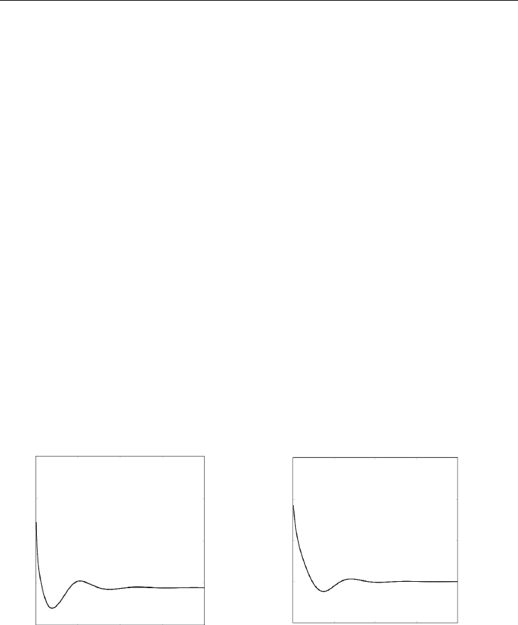
k and its initial condition. This stabilization is global. In Fig.

1 ()

t and ()t

are drawn for

()hx x x x

and

()

μς ς ς ς

for initial condition

(,,) (2,6,6)xk

=−



-2

0 7

(a)

-1

0 7

(b)

Fig. 1.

()

t and ()t

are drawn for

()hx x x x

++and

()

μς ς ς ς

++for initial

condition

(,,) (2,6,6)xk

−



. The horizontal axis is time. The vertical axis in (a) is ()t

and

in (b) is ()

t .

Automation and Robotics

The closed-loop system (17) has a one dimensional manifold of equilibria defined

by (, ) 0x

= . Every equilibrium on this manifold has one zero eigenvalue due to the

degeneracy appeared in

−



equation as a result of adaptive back-stepping design. The

stability type of equilibria on this manifold is characterized by two more eigenvalues given

by the linearization of the vector field around those equilibria. One can observe that the

arbitrary equilibrium

(0, 0, )k

∞



has two eigenvalues given by the polynomial

11 11

() 1 0,hhk

λμλμ

∞

+++−=



(18)

where

'(0)hh= and

'(0)

μμ

. The single-wedge bifurcation may take place when

10hk

∞

+− =



, and

> . This later condition is always the case as long as both

linear parts of

h and

are not simultaneously zero. We denote this critical equilibrium

with

(0,0, )



. We use the change of variables

−

⎡

⎤

⎡⎤ ⎡⎤

⎢

⎥

⎢⎥ ⎢⎥

−−

⎣⎦ ⎣⎦

⎣

⎦

(19)

Here, the column of

are the eigenvectors of the linearization matrix of the (, )x

− part of

the vector field (17) around the critical equilibrium corresponding to the eigenvalues

111

λμ

=− − < and

respectively. Such transformation keeps k



invariant. In order

to analyze the closed-loop system (17) around its critical equilibrium, we first represent the

system (17) in terms of

(,,)pqk



and then reduce the resultant system to the center

manifold. Here, the center manifold is given by

(, )pHqk=



. The center manifold is

invariant and tangent to the linear eigenspace corresponding to the eigenvalue

= .

Therefore,

pqk

∂∂

∂









(20)

The lengthy, but straightforward procedure of center manifold calculation leads to the

following truncation of the reduced system

(| , | ),

(| , | ).

qq qkqOqk

kqqOqk

ββ

⎧

=++

⎪

⎨

⎪

⎩







(21)

Here,

12 1 2

1211

11 11

,,,

μμ

ββγ

μμ

==−

(22)

Closed-Loop Feedback Systems in Automation and Robotics, Adaptive and Partial Stabilization

where,

2 ''(0)hh= and

2''(0)

. It can be observed that the reduced system (21) is

degenerate. We utilize the singular time reparametrization (Dumortier & Roussarie, 2000);

that is

= to achieve the divided out system

(| , | ),

qqkOqk

kqOqk

ββ

⎧

′

== + +

⎪

⎨

⎪

′

== +

⎪

⎩







(23)

which is generically hyperbolic around the origin. The singular time reparametrization

keeps the orbits but the direction of which are reversed when

. In order to have single-

wedge bifurcation for the closed-loop system (17), it is sufficient that the origin of the system

(23) become a node, either stable or unstable. The characteristic equation of the origin of the

system (23) is

121

λβλβγ

−

−= (24)

The sign of the discriminant of this algebraic equation is equivalent to the sign of

22 22

,ABhCh

μμω

++ − (25)

where,

42 2 2

11 11 111

,,2,44.

hB C h h h

μω μ

== = =+ (26)

The origin of the divided out system (23) is a center when

. This implies that the

center manifold (21) has a semi-center at the origin. This causes that the critical equilibrium

of the closed-loop system (17) to have a semi-center. However, when

, the origin of

the divided out system (23) is a node; therefore, the critical equilibrium of the closed-loop

system (17) undergoes a single-wedge bifurcation. It can be observed that

corresponding to the stripe

11 11

11,

hh Ahh

−+<+ <+ (27)

(,)h

− parameter space. It is worth noting that the second order derivatives of h and

control the occurrence of the single-wedge bifurcation. When

= , we have

< and there will be no single-wedge bifurcation. When

|| ( , ) ||h

is large enough, that

0.5

22111

|/(2)|2/(1/)CAh h h

μμ

+>+

, the parameter

become positive and single-

wedge bifurcation takes place. With

, the critical values of

h are

0.5

21111

2/ (1 / )

hh h

μμ

=± + , and for

, the critical values of

are

0.5

2111

2/ (1 / )

μμ

=± +

Automation and Robotics

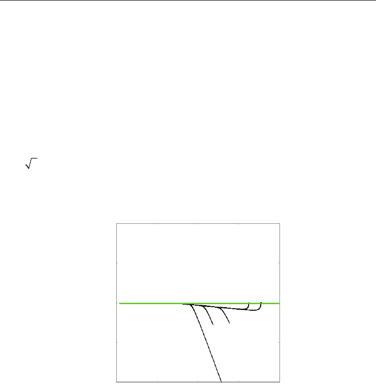
In Fig. 2, the single-wedge bifurcation appeared in the reduced system (23) is shown for the

case

() 2hx x x x=+ + and

() 2

ςςςς

++. Here

12 1

4, 0.5, 1

βγ

==−. The

wedge region is the set of all initial conditions attracting to the origin where the limit system

is unstable. The black curves are orbits converging the bifurcation point. The wedge is the

lower right area limited by the border, tick horizontal line and one of the orbits.

Remark 1: The single-wedge bifurcation generically appears due to the nonlinear terms in

feedbacks. One might argue that by applying linear feedbacks such situation can be

avoided. However, linear feedbacks are applying through devices which may introduce

some amount of nonlinearities. The width of the stripe defined by (27) depends on

h and

and is bounded by

0.5

111

4/ (1 / )hh

ημ

=+ . The linear coefficients

h and

determine

the local convergence. When they are small the convergence will slow down. One can

observe that if we expect similar rate of local convergence for both

and

, then

42/h

= approximately. For large enough

h the area where the single-wedge

bifurcation does not take place will narrow down. To extend this region one needs to slow

down the convergence process which may not be desirable. Another reason to consider this

situation is to illustrate that how such behavior happens in a simple system. In a more

complicated case, such dramatic behavior may occur generically.

-1

-0.5 0.5

Fig. 2. The single-wedge bifurcation is shown for

() 2hx x x x

++ and

() 2

μς ς ς ς

=+ +

. The horizontal axis is k



and the vertical axis is q . The tick horizontal

line represents the manifold of equilibria.

Remark 2: In our analysis, we assumed that 0

= . By some algebraic calculation, it can be

observed that including the term

with 0

≠

will only shift the value of

by the

amount of

. It can be understood from equation (21) that the limit system corresponding

∞



is unstable, but due to the linear part

∞



, the limit system will be only

unstable and finite escape time will not arise. It suggests that the closed-loop inverted