I. Ramos Arreguin (ed.) Automation and Robotics
Подождите немного. Документ загружается.

14
A Declarative Framework for Constrained
Search Problems in Manufacturing
Sitek Pawek and Wikarek Jaroslaw
Technical University of Kielce
Poland
1. Introduction
Today's highly competitive business environment makes it an absolute requirement on
behalf of the managers to continuously make the best decisions in the shortest possible time.
‘Learning from mistakes’ has left its place to ‘one strike and you're out' reality. That is, there is
no room for mistake in making decisions in this global environment. Success depends on
quickly allocating the organizational resources towards meeting the actual needs and
requirements of the customer. Decision problems involve various numeric and non-numeric
constraints, some of which are conflicting with each other. Occasionally, decision-makers do
not have complete information on the situation. Thus they perform ‘what-if’ and goal-
seeking analyses involving constraints. In order to succeed in such an unforgiving
environment, managers and decision makers need integrated 'intelligent' decision support
systems (DSS) that are capable of using a wide variety of models along with data and
information resources available to them at various internal and external repositories. In this
chapter we present the use of constraint logic programming as a tool for such decision
support systems in constrained search problems, focusing on the model representation and
analyses.
The original contribution of our approach consists of a declarative framework for
constrained search problems, developed within the constraint logic programming (CLP)
paradigm together with relational SQL database, and the development of a constraint logic
solver for scheduling problems with external resources and resource dependent processing
times in different production organization environments.
2. Constrained search problems
Constrained search problems (e.g., scheduling, planning, resource allocation, placement,
routing) appear frequently at different levels of decision in manufacturing. They are usually
characterized by technical, environmental or manpower constraints, which make them
unstructured, and in most of the cases are difficult to solve (NP-complete). Traditional
mathematical programming approaches (linear programming, integer and mixed integer
programming) are deficient in the following ways: their representation of constraints is
artificial (commonly using 0-1 variables), their computing time in the presence of many
constraints is very long (due to combinatorial explosion), and they cannot process various
constraints applied to the main problem. Thus, the most used approach consists in

Automation and Robotics
244
developing specific software, written in a procedural language like PASCAL,
BASIC or C, to
solve each particular problem. However, the use of procedural languages brings the
following well known disadvantages: the development time of the programs is very long
and the programs are very complex, hence difficult to maintain and adapt to rapid changes
of requirements.
Unlike traditional approaches, CLP provides for a natural representation of heterogeneous
constraints and allows domain-specific heuristics to be used on top of generic solving
techniques.
3. Declarative programming – SQL, CLP
Declarative programming is a term with two distinct meanings, both of which are in current
use. According to one definition, a program is ‘declarative’ if it describes what something is
like, rather than how to create it. For example, HTML, XML web pages are declarative
because they describe what the page should contain — title, text, images — but not how to
actually display the page on a computer screen. This is a different approach from imperative
programming languages such as PASCAL, C, and Java, which require the programmer to
specify an algorithm to be run. In short, imperative programs explicitly specify an algorithm
to achieve a goal, while declarative programs explicitly specify the goal and leave the
implementation of the algorithm to the support software (for example, an SQL select
statement specifies the properties of the data to be extracted from a database, not the process
of extracting the data).
According to a different definition, a program is ‘declarative’ if it is written in a purely
functional programming language, logic programming language, or constraint
programming language. The phrase "declarative language" is sometimes used to describe all
such programming languages as a group, and to contrast them against imperative
languages.
These two definitions overlap somewhat. In particular, constraint programming and, to a
lesser degree, logic programming, focus on describing the properties of the desired solution
(the what), leaving unspecified the actual algorithm that should be used to find that solution
(the how). However, most logic and constraint languages are able to describe algorithms and
implementation details, so they are not strictly declarative by the first definition.
Constraint Logic Programming (CLP) is a declarative modelling and procedural
programming environment that integrates qualitative /heuristic knowledge representation
of logic and quantitative/algorithmic reasoning into a single paradigm. Unlike traditional
approaches, CLP provides for a natural representation of heterogeneous constraints and
allows domain-specific heuristics to be used on top of generic solving techniques. The main
issue for the constrained-based approach is CSP (Constraint Satisfaction Problem). In
artificial intelligence and operation research, constraint satisfaction is the process of finding
a solution to a set of constraints. Such constraints express allowed values for variables. A
solution is therefore an evaluation of these variables that satisfies all constraints. Constraint
Satisfaction Problems (on finite domains) are typically solved using a form of search. The
most used techniques are variants of backtracking, constraint propagation and local search.
CLP as a declarative modelling and procedural programming environment is increasingly
realized as an effective tool for decision support systems (Bisdorff & Laurent, 1995; Lamma
et al., 1997; Lee & Lee 1996). Constraint Logic Programming is suitable for Decision Support
Systems (DSS) because (Liao et al., 2002; Ryu, 1998):

A Declarative Framework for Constrained Search Problems in Manufacturing
245
• CLP is a very good tool for the development of knowledge base that has expertise and
experience represented in terms of logic, rules and constraints. This tool allows the
knowledge base to be built in an incremental and accumulating way (it is suitable for
ill-structured or semi-structured decision analysis problems).
• Constraints naturally represent decisions and their inter-dependencies. Decision choices
are explicitly modelled as the domains of constraint variables.
• CLP can serve as a good integrative environment for the decision analysis that has
different kinds of model.
Decision analysis requires a number of computational facilities which this tool can provide.
4. Declarative framework for constrained search problems
There is a growing need for decision support tools capable of assisting a decision maker in
the constrained search problems in manufacturing. The most important of them are
scheduling problems and scheduling problems with resource allocation. The diversity of
scheduling problems, the existence of many specific constraints (precedence, resource,
capacity, etc.) in each problem and the efficient constraint based scheduling algorithms
make constraint logic programming a method of choice for the resolution of complex
practical problems. In constraint programming approach to decision support in scheduling
problems, the problem to be solved is represented in terms of decision variables and
constraints on these variables (Pape, 1995).
Depending on the particular applications, the variables of scheduling problems (job-shop,
flow-shop, open-shop, and project shop) can be:
• The start time and the end time of each operation.
• The set of resources assigned to each operation (if this set is not fixed).
• The capacity of a resource that is assigned to an operation (e.g. the number of workers
from a given team assigned to operation).
• The processing times (constant, variable increasing/decreasing function of starting
times or allocated resources, etc.).
The constraints of a scheduling problem include:
• Temporal and precedence constraints which define the possible values for the start and
end times of operations and the relations between the start and end time of two
operations.
• Resource constraints which define the possible set of resources for each operation.
• Capacity constraints which limit the available capacity of each resource over time.
• Problem-specific constraint which correspond to particular features of operations and
resources.
Additional variables and constraints can be included to represent optimization criteria,
preferences of the user of scheduling system, etc.
4.1 Assumptions of DSS based on declarative framework
The presented in (section 3) advantages and possibilities of CLP environment for decision
support make it interesting for decision support in constrained search problems. Building
decision support system for scheduling, covering a variety of production organization
forms, such as job-shop, flow-shop, project, multi-project etc., is especially interesting.
The following assumptions were adopted in order to design the presented scheduling
processes of decision support system (see Fig. 1.):
Automation and Robotics
246
• Problem-specific constraint which correspond to particular features of operations and
resources.
• The system should possess data structures that make its use possible in different
production organization environments (see Fig. 2.).
• The system should make it possible to schedule the whole set of tasks/jobs
simultaneously, and after a suitable schedule has been found, it should be possible to
add a new set of tasks later, and to find a suitable schedule for both sets without the
necessity to change initial schedules.
• The decisions of the systems are the answers to appropriate questions formed as CLP
predicates.
• The system should regard:
o additional resource types apart from machines, e.g. people, tools, etc,
o temporary inaccessibility of all resource types,
o resource or time depending processing times, etc.
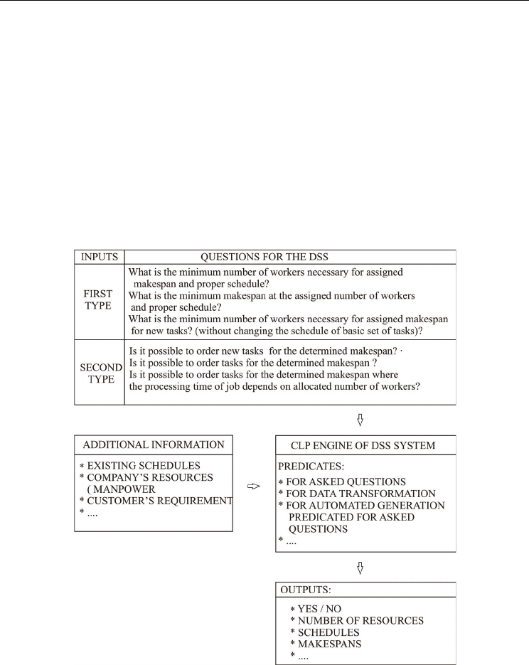
Fig. 1. Concept of DSS for scheduling problems based on declarative framework.
The range of the decisions made by the system depends on data structures and asked
questions. Thus, the system is very flexible as it is possible to ask all kinds of questions
(write all kinds of predicates). In this version of DSS the questions which can be asked are
the following:

A Declarative Framework for Constrained Search Problems in Manufacturing
247
• What is the minimum number of workers necessary for assigned makespan and proper
schedule? (predicate opc_d(L,C)).
• What is the minimum makespan at the assigned number of workers and proper
schedule? (predicate opc_g(L,C)).
• Is it possible to order new tasks (both orders and projects) for the determined
makespan? (predicate opc_s(L,C)).
• What is minimum makespan at the assigned number of workers for new tasks?
(predicate opcd_g(L,C)).
• What is the minimum number of workers necessary for assigned makespan for new
tasks? (without changing the schedule of basic set of tasks) (predicate opcd_d(L,C)).
• Is it possible to order tasks for the determined makespan ? (predicate opcd_s(L,C)).
• Is it possible to order tasks for the determined makespan where the processing time of
task depends on allocated number of workers? (predicate opcd_s1(L,C)).
L – number of workers (manpower), C=C
max
– makespan
These questions are just examples of questions that the present system can be asked. New
questions are new predicates that need to be created in CLP environment. Two types of
questions are asked in the system:
• About the existence of the solution (eg., is it possible to carry out a new task in the
particular time?, etc.).
• About a particular kind of the solution: find a suitable schedule fulfilling the
performance index, find the minimum scheduling length-makespan, find the minimum
number of workers to carry out the task, etc.
The foregoing questions can include a random set of additional renewable resources (in this
case, workers only) and refer a random number of production organization forms (job-shop,
flow-shop, open-shop, project etc.). Additionally, the presented decision support system
model implements an extra functionality which is resource dependent processing times.
Scheduling problems literature gives the processing time as constant and defined before the
tasks are realized. In practical applications the time is significantly dependent on the
amount of the allocated resources for their realization. These dependencies are usually non-
linear and can be presented as a relationship (relational database table) or function. The
system implemented the possibility of changing the time of task/job realization in relation
to the allocated number of workers. The functionality above does not call for the change of
predicates; it requires suitably prepared data describing the problem and included in the
relational database. The proposed structure of the relational database (see Fig. 2.) and the
way CLP predicates are built allow the system to generate both schedules with determined
parameters for different production organization forms, but also include allocation of
additional resources (in general case resource sets) and effects they may have on the realized
tasks.
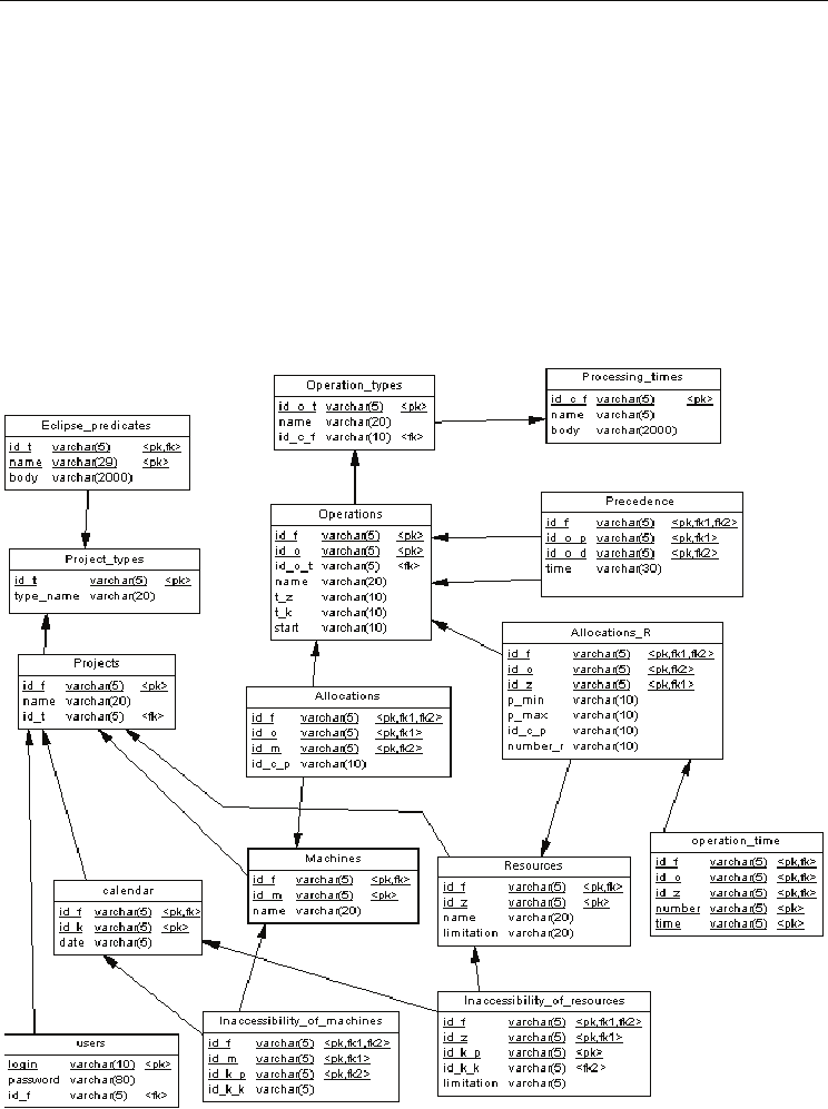
4.2 Data structures
Data structures were designed in such a way that they could be easily used to decision
problems in a variety of scheduling environments, which is job-shop, flow-shop, project or
multi-project. The obtained flexibility resulted from the use of a relational data model.
Automation and Robotics
248
Figure 2 presents the ERD (Entity Relationship Diagram) of the database that was designed
to meet the requirements of cooperation with CLP environment and to have the following
possibilities:
• Storing the data for scheduling problems and resource allocation for different types of
production organisation.
• Storing information about additional resources (e.g. labour force, tools or AGV
vehicles).
• Saving the content and parameters of CLP predicates calls.
• Generating ready scripts for a CLP engine on the basis of the existing data.
• Saving the results obtained with a CLP solver, necessary for further calculations,
visualisations or creating reports.
• Saving data about other problems within the family of constrained search problems.
Fig. 2. Schema of database of DSS for production scheduling problems (Entity Relationship
Diagram).
A Declarative Framework for Constrained Search Problems in Manufacturing
249
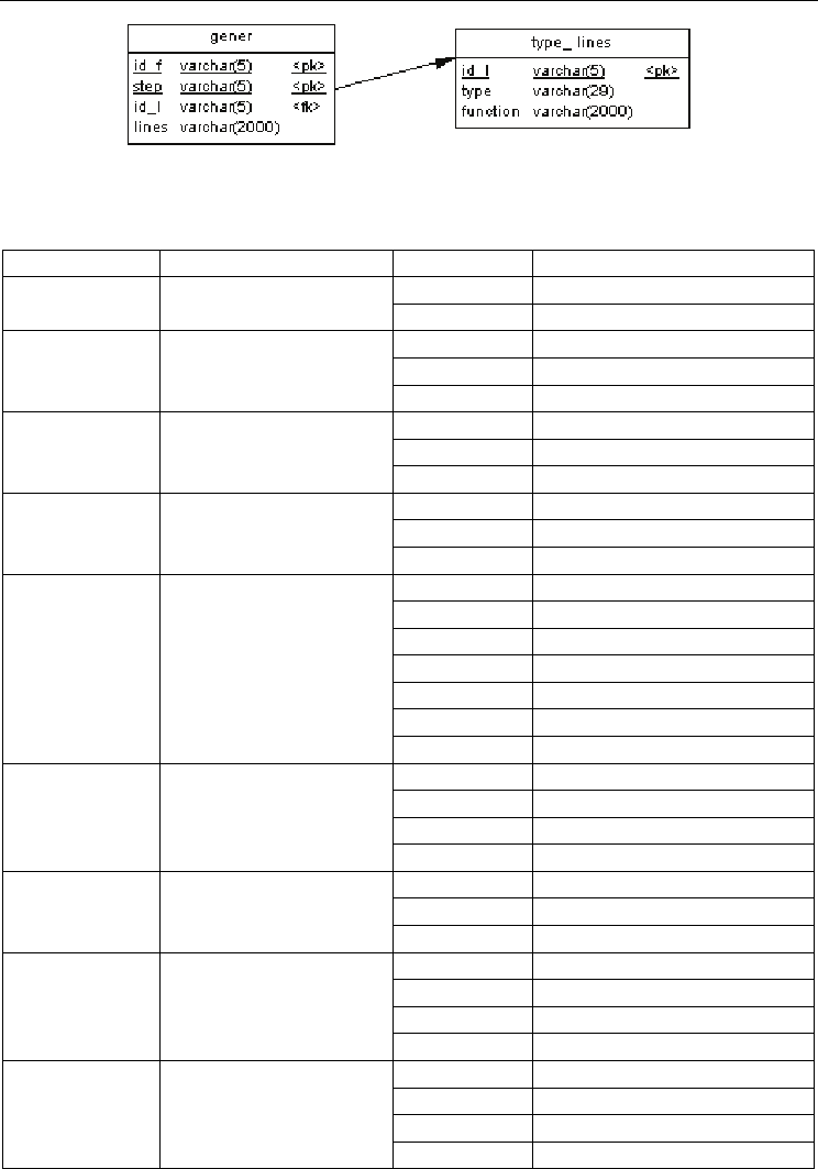
Fig. 2b. Schema of the part of database of DSS for an automatic generation CLP predicates
(Entity Relationship Diagram).
Table 1 shows the description of database structure.
Table name Table description Column Column description
id_t project_type_id
Project_types
The types of possible
projects for realization
type_name project_type_name
id_f project_id
name project_name
Projects
The specification of
separate projects in
enterprises
id_t project_type_id
id_c_f function_id
name function_name
Processing_time
s
The list of functions of
time calculation
body function_body
id_o_t operation_type_id
name operation_type_name
Opertaion_types
The list of operation
types
id_c_f function_id
id_f project_id
id_o operation_id
id_o_t operation_type_id
name operation_name
t_z release time
t_k critical time
Operations
The list of operations to
be realized
start start time
id_f project_id
id_o_p operation_id
id_o_d operation_id
Precedence
Defines the sequence of
the realized operations
time time between operations
id_f project_id
id_m machine_id
Machines
The specification of
available machines for
the operation realization
name machine_name
id_f project_id
id_o operation_id
id_m machine_id
Allocations
The allocation of
operation to machines
id_c_p parameters_of_function
id_f project_id
id_z resource_id
name resource_name
Resources
The specification of
renewable/external
resources
limitation resource_limitation

Automation and Robotics
250
Table name Table description Column Column description
id_f project_id
id_o operation_id
id_z resource_id
p_min
min number of allocated
resource
p_max
max number of allocated
resource
id_c_p parameters_of_function
Allocations_R
The allocation of
renewable/external/
additional resources to
operations
number_r number of allocated resource
id_f project_id
id_k period_number
Calendar
The specification of
planning/scheduling
periods
date starting_date
id_f project_id
id_m machine_id
id_k_p number of initial period
Inaccessibility_
of_machines
The specification of
inaccessibility of
machines
id_k_k number of final period
id_f project_id
id_z resource_id
id_k_p number of initial period
id_k_k number of final period
Inaccessibility_
of_resources
The specification of
limitation/inaccessibilit
y of resources
accessibility number of accessible resources
id_l line generation type
type type description
Type_lines
function function (in script language)
id_f project_id
step number of generation step
id_l line generation type
Gener
Describes the process of
model generation for
Eclipse
lines line to be made
id_f project_id
name name of predicate
Eclipse_predicates
The codes for the ready
predicates of Eclipse
body code of predicate
login login
password password
Users
id_f project_id
Table 1. Description of database structure.
5. Implementation of DSS based on declarative framework
We propose ECL
i
PS
e
(http://www.cs.kuleuven.ac.be, 2008, Apt & Wallace, 2007) and SQL
database as a platform to decision support in scheduling problems. ECL
i
PS
e
is a software
A Declarative Framework for Constrained Search Problems in Manufacturing
251
system - based on the CLP paradigm - for the development and deployment of constraint
programming applications. It is also ideal for developing aspects of combinatorial problem
solving, e.g. problem modelling, constraint programming, mathematical programming, and
search techniques. Its wide scope makes it a good tool for research into hybrid problem
solving methods. ECL
i
PS
e
comprises several constraint solver libraries, a high-level
modelling and control language, interfaces to third-party solvers, an integrated
development environment and interfaces for embedding into host environment. The
ECL
i
PS
e
programming language is largely backward-compatible with Prolog and supports
different dialects.
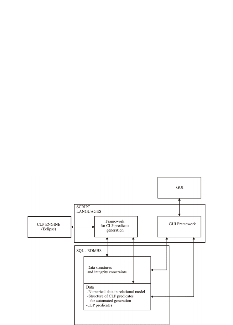
The novelty of the proposed approach is in the integration of the CLP methodology with a
commonly used relational database model. The scripts started by a CLP engine are
generated automatically on the basis of data in the database (numerical values and CLP
predicates). The proposed solution makes it possible to easily develop the system
(developing and saving in the database the content of additional CLP predicates) and to
integrate it with other computer systems based on a relational SQL database (Fig. 3.). Owing
to the developed database structure (see Fig. 2.) solving other problems of the constrained
search problems class is possible. In order to ensure an automatic generation of the
production scheduling problem model in the form of a script with CLP predicates, two
additional tables were added to the database (Fig. 2b). The gener table describes the model
schema as lines containing the model’s identity (id_f), generating step (step) and the identity
of the line type that is to be written in the CLP script (id_l) with its source (lines). The type of
the generated line is determined from the entry in the table type lines. The model (CLP
script) distinguishes lines created among others as inserting CLP predicate (line in the
eclipse_predicates table), inserting data after SQL statement, inserting a comment, heading,
etc; thus the relation between tables gener and type_lines is 1:N type (Fig. 2b.).
Fig. 3. Implementation of the declarative framework of DSS.
Automation and Robotics
252
6. Illustrative examples
After the complete implementation of the DSS into ECL
i
PS
e
and SQL environments,
computation experiments were carried out. The job-shop scheduling problem with
manpower resources (Example 1) and project –building house (Example 2) were considered.
The proposed illustrative examples cover a wide range of scheduling problems encountered
in the SMEs (Small and Medium Sized Enterprises). The examples are selected in such a way
that they how two extremely different forms of production organization; repetitive
production in the job-shop environment and the unique production including the project.
The presented methodology makes solving scheduling problems possible also in indirect
methods of production organization. Moreover, the examples are larded with problems of
constrained resources (e.g. manpower, specialized machines, etc.) and the dependence of
particular jobs processing time on the amount of the allocated resources, for instance
6.1 Example 1- the job shop scheduling
In the classical scheduling theory job processing times are constant (Example_1a). However,
there are many situations where processing time of a job depends on the starting time of the
job in queue or the amount of allocated additional resources (e.g. people) (Example_1b) etc.
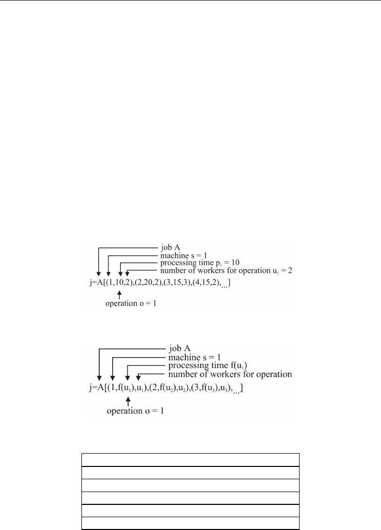
The parameters of computational examples are presented in table 2. The job data structures
are shown in Fig. 4a and Fig. 4b
Fig. 4a. Description of task (job) data structure for job-shop computational example
(Example_1a) – the constant processing times.
Fig. 4b. Description of task (job) data structure for job-shop computational example
(Example_1b) – the processing times depend on allocated number of workers.
j∈{A,B,C,D,E}, o∈{1,2,3,4,5}, s∈{1,2,3,4,5}
j=A [(1,10,2), (2,20,2), (3,15,3), (4,15,2), (5,15,1)]
j=B[(1,10,1), (2,20,1), (3,15,2), (4,15,1), (5,20,1)]
j=C[(5,15,2), (4,20,2), (3,15,1), (2,10,2), (1,20,2)]
j=D[(1,10,3), (3,15,2), (2,20,2), (4,20,1), (5,10,2)]
j=E[(5,15,2), (4,10,1), (3,15,2), (2,10,2), (1,20,1)]
Table 2. (Example_1) – constant processing times