Hager G., Wellein G. Introduction to High Performance Computing for Scientists and Engineers

Подождите немного. Документ загружается.

Shared-memory parallel programming with OpenMP 155

Listing 6.4: Fortran sentinels and conditional compilation with OpenMP combined.

1 !$ use omp_lib

2 myid=0

3 numthreads=1

4 #ifdef _OPENMP

5 !$OMP PARALLEL PRIVATE(myid)

6 myid = omp_get_thread_num()

7 !$OMP SINGLE

8 numthreads = omp_get_num_threads()

9 !$OMP END SINGLE

10 !$OMP CRITICAL

11 write(

) ’Parallel program - this is thread ’,myid,&

12 ’ of ’,numthreads

13 !$OMP END CRITICAL

14 !$OMP END PARALLEL

15 #else

16 write(

) ’Serial program’

17 #endif

all caches get updated values. This can also be initiated under program control via

the FLUSH directive, but most OpenMP worksharing and synchronization constructs

perform implicit barriers, and hence ﬂushes, at the end.

Note that compiler optimizations can prevent modiﬁed variable contents to be

seen by other threads immediately. If in doubt, use the FLUSH directive or declare

the variable as volatile (only available in C/C++ and Fortran 2003).

Thread safety

The write statement in line 11 is serialized (i.e., protected by a critical region)

so that its output does not get clobbered when multiple threads write to the console.

As a general rule, I/O operations and general OS functionality, but also common

library functions should be serialized because they may not be thread safe. A promi-

nent example is the rand() function from the C library, as it uses a static variable

to store its hidden state (the seed).

Afﬁnity

One should note that the OpenMP standard gives no hints as to how threads are

to be bound to the cores in a system, and there are no provisions for implementing

locality constraints. One cannot rely at all on the OS to make a good choice regarding

placement of threads, so it makes sense (especially on multicore architectures and

ccNUMA systems) to use OS-level tools, compiler support or library functions to

explicitly pin threads to cores. See Appendix A for technical details.

156 Introduction to High Performance Computing for Scientists and Engineers

Environment variables

Some aspects of OpenMP program execution can be inﬂuenced by environment

variables. OMP_NUM_THREADS and OMP_SCHEDULE have already been described

above.

Concerning thread-local variables, one must keep in mind that usually the OS

shell restricts the maximum size of all stack variables of its processes, and there may

also be a system limit on each thread’s stack size. This limit can be adjusted via

the OMP_STACKSIZE environment variable. Setting it to, e.g., “100M” will set a

stack size of 100MB per thread (excluding the initial program thread, whose stack

size is still set by the shell). Stack overﬂows are a frequent source of problems with

OpenMP programs.

The OpenMP standard allows for the number of active threads to dynamically

change between parallel regions in order to adapt to available system resources (dy-

namic thread number adjustment). This feature can be switched on or off by setting

the OMP_DYNAMIC environment variable to true or false, respectively. It is un-

speciﬁed what the OpenMP runtime implements as the default.

6.2 Case study: OpenMP-parallel Jacobi algorithm

The Jacobi algorithm studied in Section 3.3 can be parallelized in a straightfor-

ward way. We add a slight modiﬁcation, however: A sensible convergence criterion

shall ensure that the code actually produces a converged result. To do this we in-

troduce a new variable maxdelta, which stores the maximum absolute difference

over all lattice sites between the values before and after each sweep (see Listing 6.5).

If maxdelta drops below some threshold eps, convergence is reached.

Fortunately the OpenMP Fortran interface permits using the MAX() intrinsic

function in REDUCTION clauses, which simpliﬁes the convergence check (lines 7

and 15 in Listing 6.5). Figure 6.3 shows performance data for one, two, and four

threads on an Intel dual-socket Xeon 5160 3.0GHz node. In this node, the two cores

in a socket share a common 4MB L2 cache and a frontside bus (FSB) to the chipset.

The results exemplify several key aspects of parallel programming in multicore en-

vironments:

• With increasing N there is the expected performance breakdown when the

working set (2 ×N

×8 bytes) does not ﬁt into cache any more. This break-

down occurs at the same N for single-thread and dual-thread runs if the two

threads run in the same L2 group (ﬁlled symbols). If the threads run on dif-

ferent sockets (open symbols), this limit is a factor of

√

2 larger because the

aggregate cache size is doubled (dashed lines in Figure 6.3). The second break-

down at very large N, i.e., when two successive lattice rows exceed the L2

cache size, cannot be seen here as we use a square lattice (see Section 3.3).

• A single thread can saturate a socket’s FSB for a memory-bound situation, i.e.,

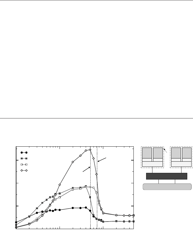
Shared-memory parallel programming with OpenMP 157

Listing 6.5: OpenMP implementation of the 2D Jacobi algorithm on an N ×N lattice, with a

convergence criterion added.

1 double precision, dimension(0:N+1,0:N+1,0:1) :: phi

2 double precision :: maxdelta,eps

3 integer :: t0,t1

4 eps = 1.d-14 ! convergence threshold

5 t0 = 0 ; t1 = 1

6 maxdelta = 2.d0

eps

7 do while(maxdelta.gt.eps)

8 maxdelta = 0.d0

9 !$OMP PARALLEL DO REDUCTION(max:maxdelta)

10 do k = 1,N

11 do i = 1,N

12 ! four flops, one store, four loads

13 phi(i,k,t1) = ( phi(i+1,k,t0) + phi(i-1,k,t0)

14 + phi(i,k+1,t0) + phi(i,k-1,t0) )

0.25

15 maxdelta = max(maxdelta,abs(phi(i,k,t1)-phi(i,k,t0)))

16 enddo

17 enddo

18 !$OMP END PARALLEL DO

19 ! swap arrays

20 i = t0 ; t0=t1 ; t1=i

21 enddo

10 100 1000

500

1000

1500

Performance [MLUPs/sec]

1 thread

2 threads, 1 socket

2 threads, 2 sockets

4 threads

8 MB L2

4 MB L2

socket

32k L1D 32k L1D 32k L1D 32k L1D

Chipset

Memory

P P P P

4MB L2 4MB L2

Figure 6.3: Performance versus problem size of a 2D Jacobi solver on an N ×N lattice with

OpenMP parallelization at one, two, and four threads on an Intel dual-core dual-socket Xeon

5160 node at 3.0GHz (right). For two threads, there is a choice to place them on one socket

(ﬁlled squares) or on different sockets (open squares).

158 Introduction to High Performance Computing for Scientists and Engineers

at large N. Running two threads on the same socket has no beneﬁt whatsoever

in this limit because contention will occur on the frontside bus. Adding a sec-

ond socket gives an 80% boost, as two FSBs become available. Scalability is

not perfect because of deﬁciencies in the chipset and FSB architecture. Note

that bandwidth scalability behavior on all memory hierarchy levels is strongly

architecture-dependent; there are multicore chips on which it takes two or more

threads to saturate the memory interface.

• With two threads, the maximum in-cache performance is the same, no matter

whether they run on the same or on different sockets (ﬁlled vs. open squares).

This indicates that the shared L2 cache can saturate the bandwidth demands

of both cores in its group. Note, however, that three of the four loads in the

Jacobi kernel are satisﬁed from L1 cache (see Section 3.3 for an analysis of

bandwidth requirements). Performance prediction can be delicate under such

conditions [M41, M44].

• At N < 50, the location of threads is more important for performance than

their number, although the problem ﬁts into the aggregate L1 caches. Using

two sockets is roughly a factor of two slower in this case. The reason is that

OpenMP overhead like the barrier synchronization at the end of the OpenMP

worksharing loop dominates execution time for small N. See Section 7.2 for

more information on this problem and how to ameliorate its consequences.

Explaining the performance characteristics of this bandwidth-limited algorithm re-

quires a good understanding of the underlying parallel hardware, including issues

speciﬁc to multicore chips. Future multicore designs will probably be more “aniso-

tropic” (see, e.g., Figure 1.17) and show a richer, multilevel cache group structure,

making it harder to understand performance features of parallel codes [M41].

6.3 Advanced OpenMP: Wavefront parallelization

Up to now we have only encountered problems where OpenMP parallelization

was more or less straightforward because the important loops comprised indepen-

dent iterations. However, in the presence of loop-carried dependencies, which also

inhibit pipelining in some cases (see Section 1.2.3), writing a simple worksharing

directive in front of a loop leads to unpredictable results. A typical example is the

Gauss–Seidel algorithm, which can be used for solving systems of linear equations

or boundary value problems, and which is also widely employed as a smoother com-

ponent in multigrid methods. Listing 6.6 shows a possible serial implementation in

three spatial dimensions. Like the Jacobi algorithm introduced in Section 3.3, this

code solves for the steady state, but there are no separate arrays for the current and

the next time step; a stencil update at (i, j,k) directly re-uses the three neighboring

sites with smaller coordinates. As those have been updated in the very same sweep

Shared-memory parallel programming with OpenMP 159

Listing 6.6: A straightforward implementation of the Gauss–Seidel algorithm in three dimen-

sions. The highlighted references cause loop-carried dependencies.

1 double precision, parameter :: osth=1/6.d0

2 do it=1,itmax ! number of iterations (sweeps)

3 ! not parallelizable right away

4 do k=1,kmax

5 do j=1,jmax

6 do i=1,imax

7 phi(i,j,k) = ( phi(i-1,j,k) + phi(i+1,j,k)

8 + phi(i,j-1,k) + phi(i,j+1,k)

9 + phi(i,j,k-1) + phi(i,j,k+1) )

osth

10 enddo

11 enddo

12 enddo

13 enddo

before, the Gauss–Seidel algorithm has fundamentally different convergence proper-

ties as compared to Jacobi (Stein-Rosenberg Theorem).

Parallelization of the Jacobi algorithm is straightforward (see the previous sec-

tion) because all updates of a sweep go to a different array, but this is not the case

here. Indeed, just writing a PARALLEL DO directive in front of the k loop would

lead to race conditions and yield (wrong) results that most probably vary from run to

run.

Still it is possible to parallelize the code with OpenMP. The key idea is to ﬁnd a

way of traversing the lattice that fulﬁlls the dependency constraints imposed by the

stencil update. Figures 6.4 and 6.5 show how this can be achieved: Instead of simply

cutting the k dimension into chunks to be processed by OpenMP threads, a wavefront

travels through the lattice in k direction. The dimension along which to parallelize

is j, and each of the t threads T

...T

t−1

gets assigned a consecutive chunk of size

max

/t along j. This divides the lattice into blocks of size i

max

× j

max

/t ×1. The very

ﬁrst block with the lowest k coordinate can only be updated by a single thread (T

which forms a “wavefront” by itself (W

in Figure 6.4). All other threads have to

wait in a barrier until this block is ﬁnished. After that, the second wavefront (W

)

can commence, this time with two threads (T

and T

), working on two blocks in

parallel. After another barrier, W

starts with three threads, and so forth. W

is the

ﬁrst wavefront to actually utilize all threads, ending the so-called wind-up phase.

Some time (t wavefronts) before the sweep is complete, the wind-down phase begins

and the number of working threads is decreased with each successive wavefront. The

block with the largest k and j coordinates is ﬁnally updated by a single-thread (T

t−1

)

wavefront W

again. In the end, n= k

max

+t −1 wavefronts have traversed the lattice

in a “pipeline parallel” pattern. Of those, 2(t −1) have utilized less than t threads.

The whole scheme can thus only be load balanced if k

max

≫t.

Listing 6.7 shows a possible implementation of this algorithm. We assume here

for simplicity that j

max

is a multiple of the number of threads. Variable l counts the

160 Introduction to High Performance Computing for Scientists and Engineers

max

j /t

Figure 6.4: Pipeline parallel processing (PPP), a.k.a. wavefront parallelization, for the Gauss–

Seidel algorithm in 3D (wind-up phase). In order to fulﬁll the dependency constraints of each

stencil update, successive wavefronts (W

,...,W

) must be performed consecutively, but

multiple threads can work in parallel on each individual wavefront. Up until the end of the

wind-up phase, only a subset of all t threads can participate.

Figure 6.5: Wavefront parallelization for the Gauss–Seidel algorithm in 3D (full pipeline

phase). All t threads participate. Wavefront W

is shown as an example.

Shared-memory parallel programming with OpenMP 161

Listing 6.7: The wavefront-parallel Gauss–Seidel algorithm inthree dimensions.Loop-carried

dependencies are still present, but threads can work in parallel.

1 !$OMP PARALLEL PRIVATE(k,j,i,jStart,jEnd,threadID)

2 threadID=OMP_GET_THREAD_NUM()

3 !$OMP SINGLE

4 numThreads=OMP_GET_NUM_THREADS()

5 !$OMP END SINGLE

6 jStart=jmax/numThreads

threadID

7 jEnd=jStart+jmax/numThreads ! jmax is amultiple of numThreads

8 do l=1,kmax+numThreads-1

9 k=l-threadID

10 if((k.ge.1).and.(k.le.kmax)) then

11 do j=jStart,jEnd ! this is the actual parallel loop

12 do i=1,iMax

13 phi(i,j,k) = ( phi(i-1,j,k) + phi(i+1,j,k)

14 + phi(i,j-1,k) + phi(i,j+1,k)

15 + phi(i,j,k-1) + phi(i,j,k+1) )

osth

16 enddo

17 enddo

18 endif

19 !$OMP BARRIER

20 enddo

21 !$OMP END PARALLEL

wavefronts, and k is the current k coordinate for each thread. The OpenMP barrier

in line 19 is the point where all threads (including possible idle threads) synchronize

after a wavefront has been completed.

We have ignored possible scalar optimizations like outer loop unrolling (see the

order of site updates illustrated in the T

block of Figure 6.4). Note that the stencil

update is unchanged from the original version, so there are still loop-carried depen-

dencies. These inhibit fully pipelined execution of the inner loop, but this may be of

minor importance if performance is bound by memory bandwidth. See Problem 6.6

for an alternative solution that enables pipelining (and thus vectorization).

Wavefront methods are of utmost importance in High Performance Computing,

for massively parallel applications [L76, L78] as well as for optimizing shared-

memory codes [O52, O59]. Wavefronts are a natural extension of the pipelining

scheme to medium- and coarse-grained parallelism. Unfortunately, mainstream pro-

gramming languages and parallelization paradigms do not as of now contain any

direct support for it. Furthermore, although dependency analysis is a major part of

the optimization stage in any modern compiler, very few current compilers are able

to perform automatic wavefront parallelization [O59].

Note that stencil algorithms (for which Gauss–Seidel and Jacobi are just two

simple examples) are core components in a lot of simulation codes and PDE solvers.

Many optimization, parallelization, and vectorization techniques have been devised

over the past decades, and there is a vast amount of literature available. More infor-

mation can be found in the references [O60, O61, O62, O63].

162 Introduction to High Performance Computing for Scientists and Engineers

Problems

For solutions see page 298ff.

6.1 OpenMP correctness. What is wrong with this OpenMP-parallel Fortran 90

code?

1 double precision, dimension(0:360) :: a

3 !$OMP PARALLEL DO

4 do i=0,360

5 call f(dble(i)/360

PI, a(i))

6 enddo

7 !$OMP END PARALLEL DO

9 ...

11 subroutine f(arg, ret)

12 double precision :: arg, ret, noise=1.d-6

13 ret = SIN(arg) + noise

14 noise = -noise

15 return

16 end subroutine

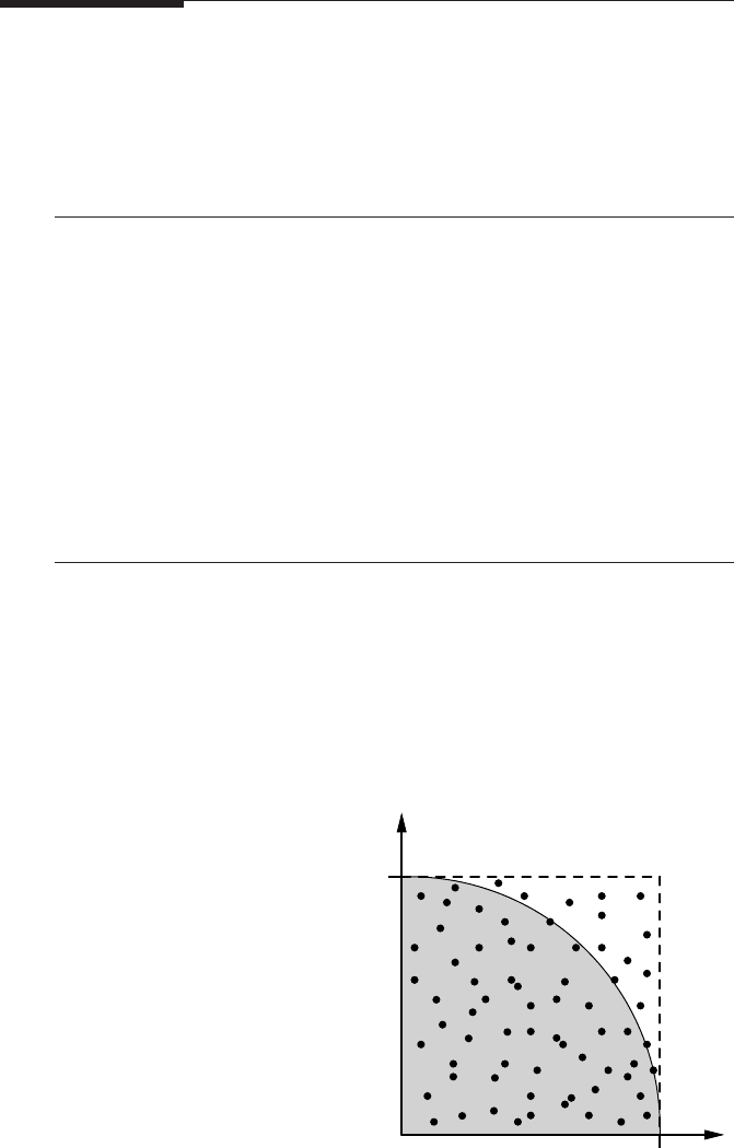
6.2

by Monte Carlo. The quarter circle in the ﬁrst quadrant with origin at (0,0)

and radius 1 has an area of

/4. Look at the random number pairs in [0,1] ×

[0,1]. The probability that such a point lies inside the quarter circle is

/4, so

given enough statistics we are able to calculate

using this so-called Monte

Carlo method (see Figure 6.6). Write a parallel OpenMP program that per-

forms this task. Use a suitable subroutine to get separate random number se-

Figure 6.6: Calculating

by a Monte Carlo

method (see Problem 6.2). The probability

that a random point in the unit square lies

inside the quarter circle is

/4.

Shared-memory parallel programming with OpenMP 163

quences for all threads. Make sure that adding more threads in a weak scaling

scenario actually improves statistics.

6.3 Disentangling critical regions. In Section 6.1.4 we demonstrated the use of

named critical regions to prevent deadlocks. Which simple modiﬁcation of the

example code would have made named the names obsolete?

6.4 Synchronization perils. What is wrong with this code?

1 !$OMP PARALLEL DO SCHEDULE(STATIC) REDUCTION(+:sum)

2 do i=1,N

3 call do_some_big_stuff(i,x)

4 sum = sum + x

5 call write_result_to_file(omp_get_thread_num(),x)

6 !$OMP BARRIER

7 enddo

8 !$OMP END PARALLEL DO

6.5 Unparallelizable? (This problem appeared on the ofﬁcial OpenMP mailing list

in 2007.) Parallelize the loop in the following piece of code using OpenMP:

1 double precision, parameter :: up = 1.00001d0

2 double precision :: Sn

3 double precision, dimension(0:len) :: opt

5 Sn = 1.d0

6 do n = 0,len

7 opt(n) = Sn

8 Sn = Sn

9 enddo

Simply writing an OpenMP worksharing directive in front of the loop will not

work because there is a loop-carried dependency: Each iteration depends on

the result from the previous one. The parallelized code should work indepen-

dently of the OpenMP schedule used. Try to avoid — as far as possible —

expensive operations that might impact serial performance.

To solve this problem you may want to consider using the FIRSTPRIVATE

and LASTPRIVATE OpenMP clauses. LASTPRIVATE can only be applied

to a worksharing loop construct, and has the effect that the listed variables’

values are copied from the lexically last loop iteration to the global variable

when the parallel loop exits.

6.6 Gauss–Seidel pipelined. Devise a reformulation of the Gauss–Seidel sweep

(Listing 6.6) so that the inner loop does not contain loop-carried dependen-

cies any more. Hint: Choose some arbitrary site from the lattice and visualize

all other sites that can be updated at the same time, obeying the dependency

constraints. What would be the performance impact of this formulation on

cache-based processors and vector processors (see Section 1.6)?