Goldreich O. P, NP, and NP-Completeness. The Basics of Computational Complexity
Подождите немного. Документ загружается.

1.3 Uniform Models (Algorithms) 9
Organization of Section 1.3. We start, in Section 1.3.1, with a general and
abstract discussion of the notion of computation. Next, in Section 1.3.2,we
provide a high-level description of the model of Turing machines. This is done
merely for the sake of providing a concrete model that supports the study
of computation and its complexity, whereas the material in this book will
not depend on the specifics of this model. In Section 1.3.3 and Section 1.3.4
we discuss two fundamental properties of any reasonable model of computa-
tion: the existence of uncomputable functions and the existence of universal
computations. The time (and space) complexity of computation is defined in
Section 1.3.5. We also discuss oracle machines and restricted models of com-
putation (in Section 1.3.6 and Section 1.3.7, respectively).
1.3.1 Overview and General Principles
Before being formal, let us offer a general and abstract description of the
notion of computation. This description applies both to artificial processes
(taking place in computers) and to processes that are aimed at modeling the
evolution of the natural reality (be it physical, biological, or even social).
A
computation is a process that modifies an environment via repeated appli-
cations of a predetermined
rule. The key restriction is that this rule is simple:
In each application it depends and affects only a (small) portion of the envi-
ronment, called the
active zone. We contrast the a priori bounded size of the
active zone (and of the modification rule) with the a priori unbounded size of
the entire environment. We note that although each application of the rule has a
very limited effect, the effect of many applications of the rule may be very com-
plex. Put in other words, a computation may modify the relevant environment
in a very complex way, although it is merely a process of repeatedly applying
a simple rule.
As hinted, the notion of computation can be used to model the “mechanical”
aspects of the natural reality, that is, the rules that determine the evolution of
the reality (rather than the specific state of the reality at a specific time). In this
case, the starting point of the study is the actual evolution process that takes
place in the natural reality, and the goal of the study is finding the (computation)
rule that underlies this natural process. In a sense, the goal of science at large
can be phrased as finding (simple) rules that govern various aspects of reality
(or rather one’s abstraction of these aspects of reality).
Our focus, however, is on artificial computation rules designed by humans
in order to achieve specific desired effects on a corresponding artificial environ-
ment. Thus, our starting point is a desired functionality, and our aim is to design
10 1 Computational Tasks and Models
computation rules that effect it. Such a computation rule is referred to as an
algorithm. Loosely speaking, an algorithm corresponds to a computer program
written in a high-level (abstract) programming language. Let us elaborate.
We are interested in the transformation of the environment as effected by
the computational process (or the algorithm). Throughout (almost all of) this
book, we will assume that, when invoked on any finite initial environment, the
computation halts after a finite number of steps. Typically, the initial environ-
ment to which the computation is applied encodes an
input string, and the end
environment (i.e., at termination of the computation) encodes an
output string.
We consider the mapping from inputs to outputs induced by the computation;
that is, for each possible input x, we consider the output y obtained at the end
of a computation initiated with input x, and say that the computation maps
input x to output y. Thus, a computation rule (or an algorithm) determines a
function (computed by it): This function is exactly the aforementioned mapping
of inputs to outputs.
In the rest of this book (i.e., outside the current chapter), we will also consider
the number of steps (i.e., applications of the rule) taken by the computation
on each possible input. The latter function is called the
time complexity of the
computational process (or algorithm). While time complexity is defined per
input, we will often considers it per input length, taking the maximum over all
inputs of the same length.
In order to define computation (and computation time) rigorously, one needs
to specify some model of computation, that is, provide a concrete definition of
environments and a class of rules that may be applied to them. Such a model
corresponds to an abstraction of a real computer (be it a PC, mainframe, or
network of computers). One simple abstract model that is commonly used is that
of Turing machines (see Section 1.3.2). Thus, specific algorithms are typically
formalized by corresponding Turing machines (and their time complexity is
represented by the time complexity of the corresponding Turing machines).
We stress, however, that almost all results in the theory of computation hold
regardless of the specific computational model used, as long as it is “reasonable”
(i.e., satisfies the aforementioned simplicity condition and can perform some
apparently simple computations).
What is being Computed? The foregoing discussion has implicitly referred
to algorithms (i.e., computational processes) as means of computing functions.
Specifically, an algorithm A computes the function f
A
:{0, 1}
∗
→{0, 1}
∗
∪{⊥}
defined by f
A
(x) =y if, when invoked on input x, algorithm A halts with output
y. However, algorithms can also serve as means of “solving search problems”
or “making decisions” (as in Definitions 1.1 and 1.2). Specifically, we will say
1.3 Uniform Models (Algorithms) 11
that algorithm A solves the search problem of R (resp., decides membership in
S)iff
A
solves the search problem of R (resp., decides membership in S). In
the rest of this exposition we associate the algorithm A with the function f
A
computed by it; that is, we write A(x) instead of f
A
(x). For the sake of future
reference, we summarize the foregoing discussion in a definition.
Definition 1.3 (algorithms as problem solvers): We denote by A(x) the output
of algorithm A on input x. Algorithm A
solves the search problem R (resp., the
decision problem S) if A, viewed as a function, solves R (resp., S).
1.3.2 A Concrete Model: Turing Machines
The model of Turing machines offers a relatively simple formulation of the
notion of an algorithm. The fact that the model is very simple complicates
the design of machines that solve problems of interest, but makes the analysis
of such machines simpler. Since the focus of Complexity Theory is on the
analysis of machines and not on their design, the trade-off offered by this
model is suitable for our purposes. We stress again that the model is merely
used as a concrete formulation of the intuitive notion of an algorithm, whereas
we actually care about the intuitive notion and not about its formulation. In
particular, all results mentioned in this book hold for any other “reasonable”
formulation of the notion of an algorithm.
The model of Turing machines provides only an extremely coarse description
of real-life computers. Indeed, Turing machines are not meant to provide an
accurate portrayal of real-life computers, but rather to capture their inherent
limitations and abilities (i.e., a computational task can be solved by a real-life
computer if and only if it can be solved by a Turing machine). In comparison to
real-life computers, the model of Turing machines is extremely oversimplified
and abstracts away many issues that are of great concern to computer practice.
However, these issues are irrelevant to the higher-level questions addressed
by Complexity Theory. Indeed, as usual, good practice requires more refined
understanding than the one provided by a good theory, but one should first
provide the latter.
Historically, the model of Turing machines was invented before modern
computers were even built, and was meant to provide a concrete model of
computation and a definition of computable functions.
2
Indeed, this concrete
2
In contrast, the abstract definition of “recursive functions” yields a class of “computable”
functions without referring to any model of computation (but rather based on the intuition that
any such model should support recursive functional composition).

12 1 Computational Tasks and Models
33222 0
33222 10
b
3
b
5
5
--------
--------
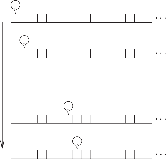
Figure 1.1. A single step by a Turing machine.
model clarified fundamental properties of computable functions and plays a
key role in defining the complexity of computable functions.
The model of Turing machines was envisioned as an abstraction of the
process of an algebraic computation carried out by a human using a sheet of
paper. In such a process, at each time, the human looks at some location on the
paper, and depending on what he/she sees and what he/she has in mind (which
is little . . . ), he/she modifies the contents of this location and shifts his/her look
to an adjacent location.
1.3.2.1 The Actual Model
Following is a high-level description of the model of Turing machines. While
this description should suffice for our purposes, more detailed (low-level)
descriptions can be found in numerous textbooks (e.g., [30]). Recall that, in
order to describe a computational model, we need to specify the set of possible
environments, the set of machines (or computation rules), and the effect of
applying such a rule on an environment.
The Environment. The main component in the environment of a Turing
machine is an infinite sequence of
cells, each capable of holding a single
symbol (i.e., member of a finite set ⊃{0, 1}). This sequence is envisioned as
starting at a leftmost cell, and extending infinitely to the right (cf. Figure 1.1).
In addition, the environment contains the
current location of the machine on
this sequence, and the
internal state of the machine (which is a member of a
finite set Q). The aforementioned sequence of cells is called the
tape, and its
contents combined with the machine’s location and its internal state is called
the
instantaneous configuration of the machine.
1.3 Uniform Models (Algorithms) 13
The Machine Itself (i.e., the Computation Rule). The main component in
the Turing machine itself is a finite rule (i.e., a finite function) called the
transition function, which is defined over the set of all possible symbol-state pairs.
Specifically, the transition function is a mapping from × Q to × Q ×
{−1, 0, +1}, where {−1, +1, 0} correspond to a movement instruction (which
is either “left” or “right” or “stay,” respectively). In addition, the machine’s
description specifies an initial state and a halting state, and the computation of
the machine halts when the machine enters its halting state. (Envisioning the
tape as in Figure 1.1, we use the convention by which if the machine ever tries
to move left of the end of the tape, then it is considered to have halted.)
We stress that in contrast to the finite description of the machine, the tape
has an a priori unbounded length (and is considered, for simplicity, as being
infinite).
A Single Application of the Computation Rule. A single computation step
of such a Turing machine depends on its current location on the tape, on the
contents of the corresponding cell, and on the internal state of the machine.
Based on the latter two elements, the transition function determines a new
symbol-state pair as well as a movement instruction (i.e., “left” or “right” or
“stay”). The machine modifies the contents of the said cell and its internal
state accordingly, and moves as directed. That is, suppose that the machine
is in state q and resides in a cell containing the symbol σ , and suppose that
the transition function maps (σ, q)to(σ
,q
,D). Then, the machine modifies
the contents of the said cell to σ
, modifies its internal state to q
, and moves
one cell in direction D. Figure 1.1 shows a single step of a Turing machine
that, when in state “b” and seeing a binary symbol σ ∈{0, 1}, replaces σ with
the symbol σ + 2, maintains its internal state, and moves one position to the
right.
3
Formally, we define the successive configuration function that maps each
instantaneous configuration to the one resulting by letting the machine take a
single step. This function modifies its argument in a very minor manner, as
described in the foregoing paragraph; that is, the contents of at most one cell
(i.e., at which the machine currently resides) is changed, and in addition the
internal state of the machine and its location may change, too.
3
Figure 1.1 corresponds to a machine that, when in the initial state (i.e., “a”), replaces the
symbol σ ∈{0, 1} by σ + 4, modifies its internal state to “b,” and moves one position to the
right. (See also Figure 1.2, which depicts multiple steps of this machine.) Indeed, “marking” the
leftmost cell (in order to allow for recognizing it in the future) is a common practice in the
design of Turing machines.
14 1 Computational Tasks and Models
Providing a concrete representation of the successive configuration function
requires providing a concrete representation of instantaneous configurations.
For example, we may represent each instantaneous configuration of a machine
with symbol set and state set Q as a triple (α, q, i), where α ∈
∗
, q ∈ Q and
i ∈{1, 2,...,|α|}.LetT : × Q → × Q ×{−1, 0, +1} be the transition
function of the machine. Then, the successive configuration function maps
(α, q, i)to(α
,q
,i + d) such that α
differs from α only in the i
th
location,
which is determined according to the first element in T (α
i
,q). The new state
(i.e., q
) and the movement (i.e., d) are determined by the other two elements
of T (α
i
,q). Specifically, except for some pathological cases, the successive
configuration function maps (α, q, i)to(α
,q
,i + d) if and only if T (α
i
,q) =
(α
i
,q
,d) and α
j
= α
j
for every j = i, where α
j
(resp., α
j
) denotes the j
th
symbol of α (resp., α
). The aforementioned pathological cases refer to cases
in which the machine resides in one of the “boundary locations” and needs to
move farther in that direction. One such case is the case that i = 1 and d =−1,
which causes the machine to halt (rather than move left of the left boundary of
the tape). The opposite case refers to i =|α| and d =+1, where the machine
moves to the right of the rightmost non-blank symbol, which is represented by
extending α
with a blank symbol “-” (i.e., |α
|=|α|+1 and α
|α|+1
= -).
Initial and Final Environments. The initial environment (or configuration)
of a Turing machine consists of the machine residing in the first (i.e., leftmost)
cell and being in its initial state. Typically, one also mandates that in the initial
configuration, a prefix of the tape’s cells holds bit values, which concatenated
together are considered the
input, and the rest of the tape’s cells hold a special
(“blank”) symbol (which in Figures 1.1 and 1.2 is denoted by “-”). Thus, the
initial configuration of a Turing machine has a finite (explicit) description. Once
the machine halts, the
output is defined as the contents of the cells that are to
the left of its location (at termination time).
4
Note, however, that the machine
need not halt at all (when invoked on some initial environment).
5
Thus, each
machine defines a (possibly partial) function mapping inputs to outputs, called
the
function computed by the machine. That is, the function computed by machine
M maps x to y if, when invoked on input x, machine M halts with output y,
and is undefined on x if machine M does halt on input x.
4
By an alternative convention, the machine must halt when residing in the leftmost cell, and the
output is defined as the maximal prefix of the tape contents that contains only bit values. In such
a case, the special non-Boolean output ⊥ is indicated by the machine’s state (and indeed in this
case the set of states, Q, contains several halting states).
5
A simple example is a machine that “loops forever” (i.e., it remains in the same state and the
same location regardless of what it reads). Recall, however, that we shall be mainly interested in
machines that do halt after a finite number of steps (when invoked on any initial environment).
1.3 Uniform Models (Algorithms) 15
01--------
0-5-------
b
a
111000
111000
3322201
b
5--------
3322203
b
-5-------
Figure 1.2. Multiple steps of the machine depicted in Figure 1.1.
As stated up front, the Turing machine model is only meant to provide
an extremely coarse portrayal of real-life computers. However, the model is
intended to reflect the inherent limitations and abilities of real-life computers.
Thus, it is important to verify that the Turing machine model is exactly as pow-
erful as a model that provides a more faithful portrayal of real-life computers
(see the “sanity check” in §1.3.2.2); that is, a function can be computed by a
Turing machine if and only if it is computable by a machine of the latter model.
For starters, one may prove that a function can be computed by a single-tape
Turing machine if and only if it is computable by a multi-tape (e.g., two-tape)
Turing machine (as defined next); see Exercise 1.3.
Multi-tape Turing Machines. We comment that in most expositions, one
refers to the location of the “head of the machine” on the tape (rather than to
the “location of the machine on the tape”). The standard terminology is more
intuitive when extending the basic model, which refers to a single tape, to a
16 1 Computational Tasks and Models
model that supports a constant number of tapes. In the corresponding model of
so-called
multi-tape machines, the machine maintains a single head on each such
tape, and each step of the machine depends on and effects the cells that are at
the machine’s head location on each tape. The input is given on one designated
tape, and the output is required to appear on some other designated tape. As
we shall see in Section 1.3.5, the extension of the model to multi-tape Turing
machines is crucial to the definition of space complexity. A less fundamental
advantage of the model of multi-tape Turing machines is that it is easier to
design multi-tape Turing machines that compute functions of interest (see, e.g.,
Exercise 1.4).
1.3.2.2 The Church-Turing Thesis
The entire point of the model of Turing machines is its simplicity. That is, in
comparison to more “realistic” models of computation, it is simpler to formulate
the model of Turing machines and to analyze machines in this model. The
Church-Turing Thesis asserts that nothing is lost by considering the Turing
machine model: A function can be computed by some Turing machine if and
only if it can be computed by some machine of any other “reasonable and
general” model of computation.
This is a thesis, rather than a theorem, because it refers to an intuitive notion
(i.e., the notion of a reasonable and general model of computation) that is
left undefined on purpose. The model should be reasonable in the sense that it
should allow only computation rules that are “simple” in some intuitive sense.
For example, we should be able to envision a mechanical implementation
of these computation rules. On the other hand, the model should allow the
computation of “simple” functions that are definitely computable according
to our intuition. At the very least, the model should allow the emulatation of
Turing machines (i.e., computation of the function that, given a description of
a Turing machine and an instantaneous configuration, returns the successive
configuration).
A Philosophical Comment. The fact that a thesis is used to link an intuitive
concept to a formal definition is common practice in any science (or, more
broadly, in any attempt to reason rigorously about intuitive concepts). Any
attempt to rigorously define an intuitive concept yields a formal definition that
necessarily differs from the original intuition, and the question of correspon-
dence between these two objects arises. This question can never be rigorously
treated because one of the objects that it relates to is undefined. That is, the
question of correspondence between the intuition and the definition always
1.3 Uniform Models (Algorithms) 17
transcends a rigorous treatment (i.e., it always belongs to the domain of the
intuition).
A Sanity Check: Turing Machines can Emulate an Abstract RAM. To
gain confidence in the Church-Turing Thesis, one may attempt to define an
abstract Random-Access Machine (RAM), and verify that it can be emulated
by a Turing machine. An
abstract RAM consists of an infinite number of memory
cells
, each capable of holding an integer, a finite number of similar registers,
one designated as
program counter, and a program consisting of instructions
selected from a finite set. The set of possible instructions includes the following
instructions:
r
reset(r), where r is an index of a register, results in setting the value of
register r to zero.
r
inc(r), where r is an index of a register, results in incrementing the content
of register r. Similarly
dec(r) causes a decrement.
r
load(r
1
,r
2
), where r
1
and r
2
are indices of registers, results in loading to
register r
1
the contents of the memory location m, where m is the current
contents of register r
2
.
r
store(r
1
,r
2
), stores the contents of register r
1
in the memory, analogously
to
load.
r
cond-goto(r, ), where r is an index of a register and does not exceed the
program length, results in setting the program counter to − 1 if the content
of register r is non-negative.
The program counter is incremented after the execution of each instruction,
and the next instruction to be executed by the machine is the one to which the
program counter points (and the machine halts if the program counter exceeds
the program’s length). The input to the machine may be defined as the contents
of the first n memory cells, where n is placed in a special input register, and all
other memory cells are assumed to be empty (i.e., contain blanks).
We note that the abstract RAM model (as defined) is as powerful as the
Turing machine model (see the following details). However, in order to make
the RAM model closer to real-life computers, we may augment it with addi-
tional instructions that are available on real-life computers like the instruction
add(r
1
,r
2
) (resp., mult(r
1
,r
2
)) that results in adding (resp., multiplying) the
contents of registers r
1
and r
2
(and placing the result in register r
1
). Like-
wise, we may augment the model with explicit loop-constructs (although such
constructs are easily implementable using the
cond-goto instruction).
We suggest proving that this abstract RAM can be emulated by a Turing
machine, see Exercise 1.5. We emphasize this direction of the equivalence of
18 1 Computational Tasks and Models
the two models, because the RAM model is introduced in order to convince
the reader that Turing machines are not too weak (as a model of general
computation). The fact that they are not too strong seems self-evident. Thus, it
seems pointless to prove that the RAM model can emulate Turing machines.
(Still, note that this is indeed the case, by using the RAM’s memory cells to
store the contents of the cells of the Turing machine’s tape, and holding its head
location in a special register.)
Reflections. Observe that the abstract RAM model is significantly more cum-
bersome than the Turing machine model. Furthermore, seeking a sound choice
of the instruction set (i.e., the instructions to be allowed in the model) cre-
ates a vicious cycle (because the sound guideline for such a choice should
have been allowing only instructions that correspond to “simple” operations,
whereas the latter correspond to easily computable functions . . . ). This vicious
cycle was avoided in the foregoing paragraph by trusting the reader to include
only instructions that are available in some real-life computer. (We comment
that this empirical consideration is justifiable in the current context because
our current goal is merely linking the Turing machine model with the reader’s
experience of real-life computers.)
1.3.3 Uncomputable Functions
Strictly speaking, the current subsection is not necessary for the rest of this
book, but we feel that it provides a useful perspective.
1.3.3.1 On the Existence of Uncomputable Functions
In contrast to what every layman would think, not all functions are computable.
Indeed, an important message to be communicated to the world is that not
every well-defined task can be solved by applying a “reasonable” automated
procedure (i.e., a procedure that has a simple description that can be applied to
any instance of the problem at hand). Furthermore, not only is it the case that
there exist uncomputable functions, but it is rather the case that most functions
are uncomputable. In fact, only relatively few functions are computable.
Theorem 1.4 (on the scarcity of computable functions): The set of computable
functions is countable, whereas the set of all functions (from strings to strings)
is not countable. Furthermore, the latter set has the same cardinality as the
power set of the natural numbers, which in turn has the same cardinality as the
set of real numbers.