Davim J. Paulo (editor). Machining. Fundamentals and Recent Advances

8 V.P. Astakhov and J.C. Outeiro

the velocity hodograph, associated plastic deformation and flows in this region.

Using the results of this study, one can visualize the chip cross-sectional area cut

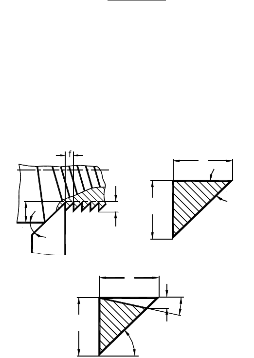
by the minor cutting edge with the help of Figure 1.4. Figure 1.4(a) shows a hypo-

thetical single-point cutting tool having

90°, i.e., practically no minor cutting

edge. Figure 1.4(b) show the cross-sectional area ABC of a tooth of the surface

profile left after this surface was machined by this tool. Real cutting tools have the

minor cutting edge with

90= °

so that the surface profile left by the cutting

tool is ADC as shown in Figure 1.4(c) and the height

h of this surface profile

(theoretical roughness) is calculated as

κκ

cot cot

(1.23)

Then, the part ABC shown in Figure 1.4(c) is cut by the minor cutting edge.

According to Zorev [3], the contribution of the cutting and deformation proc-

esses on the minor cutting edge to the overall power spent in cutting depends on

the tool minor cutting edge angle

and on the cutting feed. When the feed be-

comes significant, the minor cutting edge takes the role of the major cutting edge

so that thread cutting is the case. In real cutting tools, the tool nose radius is al-

ways made to connect the major and minor cutting edges. At moderated cutting

feeds, the crater tool wear, commonly found when machining wide variety of

steels occurs while when the feed rate becomes greater, wear of tool nose takes

(a)

(b)

= 90°

w-m

(c)

w-m

Figure 1.4. The cross-sectional area of the chip cut by the minor cutting edge: (a)

hypothetic tool having a 90° tool cutting edge angle of the minor cutting edge, (b) cross-

sectional area ABC of a tooth of the surface profile, and (c) the cross-section of the chi

by the minor cutting edge

Metal Cutting Mechanics, Finite Element Modelling 9

place [7]. This is because the energy spend due to cutting by the minor cutting

edge becomes great so that the prime mode of tool wear changes from crater to

nose wear.

An analysis of a great body of the experimental results and the results obtained by

Zorev [3] and Astakhov [7,

10] showed that, when the tool minor cutting edge angle

30 45

≤≤

, the total power should be increased by 14%, when

15 30

≤<

by 17%, when

10 15

≤<

by 20%, and when

by 23%.

1.1.5 Influence of the Cutting Speed, Depth of Cut and Cutting Feed

on Power Partition

Tables 1.1 and 1.2 show the comparison of the calculated and experimental results

for E52100 steel and aluminium alloy. Fairly good agreement between the calcu-

lated and the experimental results confirms the adequacy of the proposed method-

ology. The major advantage of the proposed methodology is that it allows not only

calculating the total power and thus the cutting force, but also provides a valuable

possibility to analyze the energy partition in the cutting system.

The results presented in Tables 1.1 and 1.2 are valid for new tools (a fresh cut-

ting edge of a cutting insert). Tool wear significantly increases the cutting force.

For steel E52100, VB

0.45 mm causes a 2.0–2.5 times increase in the cutting

force when no plastic lowering of the cutting edge [16] occurs (for cutting speeds

1 and 1.5 m/s) and a 3.0–3.5 increase when plastic lowering is the case (for cutting

speeds 3 and 4 m/s).

The proposed methodology allows accessing the absolute and relative impacts of

various variables of a metal cutting operation on the power required and thus on the

cutting force according to strictures of Equations (1.5) and (1.6). Figures 1.4−1.6

present some results for steel E52100.

Table 1.1. Comparison of the experimental and calculated results for AISI steel E52100

Cutting

Speed

(m/s)

Feed

(mm/rev)

Depth

of cut

(mm)

CCR Frequency

(kHz)

Cutting

force

Exp.

(N)

Cutting

force

Calc.

(N)

1 0.20 3 3.12 1.0 1580 1608

1.5 0.20 3 2.54 1.6 1348 1389

3 0.20 3 2.03 3.2 1076 1104

4 0.20 3 1.67 4.7 873 945

1.5 0.30 3 2.08 1.6 1562 1606

1.5 0.40 3 1.76 1.6 1640 1678

1.5 0.20 2 2.64 1.6 940 998

1.5 0.20 5 2.52 1.6 2202 2256

10 V.P. Astakhov and J.C. Outeiro

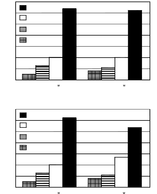
The relative impact of the cutting speed on the energy partition is shown in Fig-

ure 1.5. As seen, the power required for the plastic deformation of the layer being re-

moved in its transformation into the chip is the greatest. However, the greater the

cutting speed, the greater powers spent on the rake and flank faces of the cutting tool.

When the cutting speed is 1 m/s, the power of the plastic deformation,

P is 67%

while the power spent at the tool–chip interface,

P , is 18% and the power spent at

the tool–workpiece interface,

P , is 9%. When the cutting speed is 4 m/s,

P is

45%,

P is 25, and

P is 22%, i.e., the sum of the powers spent on the tool–chip and

tool–workpiece interfaces (

P and

P ) is greater than the power spent on the plas-

tic deformation

P . This result signifies the role of tribology in high-speed machin-

ing [7]. The power spent in the formation of new surfaces

P is 6% in both consid-

ered case, although the frequency of chip formation is much greater when

4=v m/s.

Table 1.2. Comparison of the experimental and calculated results for aluminium 2024 T6

Cutting

Speed

(m/s)

Feed

(mm/rev)

Depth

of cut

(mm)

CCR Frequency

(kHz)

Cutting

force

Exp.(N)

Cutting

force

Calc.(N)

1 0.45 4 4.96 1.0 1223 1256

3 0.45 4 3.84 2.6 1038 1076

5 0.45 4 2.65 4.2 794 854

7 0.45 4 1.92 5.8 601 625

3 0.75 4 2.82 2.6 1393 1476

3 0.50 3 3.75 2.6 906 932

3 0.50 2 3.82 2.6 632 658

3 0.30 4 3.94 2.6 787 834

70%

v=1, f=0.2, d =3

v=4, f=0.2, d =3

Figure 1.5. Relative impact of the cutting speed on the energy partition

Metal Cutting Mechanics, Finite Element Modelling 11

The relative impacts of the depth of cut and the cutting feed are shown in Fig-

ures 1.6 and 1.7. As seen in Figure 1.6, a 2.5-fold increase in the depth of cut does

not affect the energy partition. A twofold increase in the cutting feed reduces

from 62% to 54% while

P increases from 20% to 27%.

Practically the same results were obtained for aluminium. When the cutting

speed is 1 m/s, the power of the plastic deformation,

P is 67% while the power

spent at the tool–chip interface,

P is 20% and the power spent at the tool–

workpiece interface,

P , is 6% and

P is 7%. When the cutting speed is 7 m/s,

P is 50%,

P is 25,

P is 25% and

P is 6%.

1.1.6 Concluding Remarks

The proposed methodology uses the major parameters of the cutting process and

the chip compression ratio as two of the most important process outputs (in terms

of process evaluation and optimization). The apparent simplicity of the proposed

methodology is based upon a great body of theoretical and experimental studies

70%

v=1.5, f=0.2, d =2

v=1.5, f=0.2, d =5

Figure 1.6. Relative impact of the depth of cut on the energy partition.

70%

v=1.5, f=0.2, d =3

v=1.5, f=0.4, d =3

Figure 1.7. Relative impact of the cutting feed on the energy partition

12 V.P. Astakhov and J.C. Outeiro

that establish the correlations among the parameters in metal cutting. This simplic-

ity allows the use of this methodology even on the shop floor for practical evalua-

tions and optimization of machining operations.

The results of calculations indicate that the power required for the deformation

of the layer being removed is greatest in the metal cutting system within the prac-

tical cutting speed limits. When the cutting speed increases, the relative impact of

this power decreases while the powers spend at the tool–chip and tool–workpiece

interfaces increase. At high cutting speeds, the sum of these latter powers may

exceed that required for the plastic deformation of the layer being removed. This

result signifies the role of metal cutting tribology at high cutting speed.

The effects of cutting feed and the depth of cut on the energy partition seem to

be insignificant.

Although it is conclusively proven that metal cutting is the purposeful fracture

of the layer being removed [10,

17,

18], the notions and theory of traditional frac-

ture mechanics are not applicable in metal cutting studies as this analysis presup-

poses the existence of an infinitely sharp crack leading to singular crack tip fields.

In real materials, however, neither the sharpness of the crack nor the stress levels

near the crack tip region can be infinite. As an alternative approach to this singu-

larity-driven fracture approach, Barrenblatt [19] and Dugdale [20] proposed the

concept of the cohesive zone model. This model has evolved as a preferred

method to analyze fracture problems in monolithic and composite materials as

discussed by Shet and Chandra [21]. This is due to the fact that this method not

only avoids the singularity but also can be easily implemented in analytical and

numerical methods of analysis.

Although a particular cohesive zone model for metal cutting is yet to be se-

lected and justified among the many available models [21], the simplest practical

way to account for the fracture (and thus for the energy associated with the forma-

tion of new surfaces) in metal cutting is the use of the so-called cohesive energy J

(J/m

), which can be determined experimentally for any work material using

a relatively simple test [21]. Then, this energy multiplied by the area of fracture in

metal cutting, which is the area of the shear plane, defines the mechanical work

involved in the fracture and formation of new surfaces. The problem then arise of

what to do with the result obtained, i.e., how to incorporate this result in the metal

cutting model to calculate the cutting force, power and other characteristics of

a practical machining operation.

For many years, Atkins [17,

18] has argued that fracture is the case in metal

cutting even of ductile materials and that the energy associated with this fracture is

significant so it has to be accounted for in metal cutting models and calculations.

Atkins [17] and Rosa et al. [22] proposed a method of experimental determination

of the cohesive energy and incorporation this energy in the metal cutting model to

calculate the cutting force. In the authors’ opinion, however, this attempt to com-

bine the improper chip formation and thus force model [7] with the concept of

cohesive energy does not account for the real discrete metal cutting process, i.e.,

for the number of shear planes formed per unit time.

Although it is well known and depictured in any book on metal cutting that the

chip formation is discrete, i.e., at some point, a transition from one shear plane to

Metal Cutting Mechanics, Finite Element Modelling 13

the next has to happen, this simple fact has never been accounted for in the known

models of chip formation as discussed by Astakhov [7]. As the cohesive energy is

associated with a single surface of fracture, the number of surfaces of fracture that

occur per unit time is essential for the determination of the power needed for such

fracture process. In the proposed methodology, it is accounted for through the

frequency of chip formation.

Although increasing attention is played to the role of the so-called cohesive en-

ergy in metal cutting, the results obtained show that, when accounted for properly,

the relative impact of this factor is insignificant. This can be readily explained by

the very small area of fracture in metal cutting.

1.2 Finite Element Analysis (FEA)

Experimental studies in metal cutting are expensive and time consuming. More-

over, their results are valid only for the experimental conditions used and depend

greatly on the accuracy of calibration of the experimental equipment and apparatus

used. An alternative approach is numerical methods. Several numerical methods

have been used in metal cutting studies, for instance, the finite difference method,

the finite element method (FEM), the boundary element method etc. Amongst the

numerical methods, FEM is the most frequently used in metal cutting studies. The

goal of finite element analysis (FEA) is to predict the various outputs and charac-

teristics of the metal cutting process as the cutting force, stresses, temperatures,

chip geometry etc.

In the last three decades, FEM has been progressively applied to metal cutting

simulations. Starting with two-dimension simulations of the orthogonal cutting

more than two decades ago, researches progressed to three-dimensional FEM

models of the oblique cutting, capable of simulating metal cutting processes such

as turning and milling [23–25]. Increased computation power and the development

of robust calculation algorithms (thus widely availability of FEM programs) are

two major contributors to this progress. Unfortunately, this progress was not ac-

companied by new developments in metal cutting theory so the age-old problems

such as the chip formation mechanism and tribology of the contact surfaces are not

modelled properly. Therefore, although these FEM simulations can provide de-

tailed information about the distribution of stress, deformations, temperatures and

residual tensions, in the deformation zone the above referred problems raise ques-

tions about the validity of such information.

Applying FEM, one should clearly realize that the results will not contain more

physics than the inputs. In other words, if the model and its boundary conditions

are not represented adequately with physically justified assumptions and simplifi-

cations, then one should not expect meaningful results.

This section aims to present a brief analysis of some basic aspects of FEM used

in metal cutting simulations. A bibliographical review of the FEM applied to the

simulation of metal cutting is presented in [26].

14 V.P. Astakhov and J.C. Outeiro

1.2.1 Numerical Formulations

Two major numerical formulations are used in finite element (FE) simulations:

Lagrangian and Eulerian. In the Lagrangian formulation, broadly used in prob-

lems related to mechanics of solids, the FE mesh is constituted by elements that

cover exactly the whole of the region of the body under analysis. These elements

are attached to the body and thus they follow its deformation. This formulation is

particularly convenient when unconstrained flow of material is involved, i.e.,

when its boundaries are in frequent mutation. In this case, the FE mesh covers the

real contour of the body with sufficient accuracy. On the other hand, the Eulerian

formulation is more suitable for fluid-flow problems involving a control volume.

In this method, the mesh is constituted of elements that are fixed in the space and

cover the control volume. The variables under analysis are calculated at fixed

spatial location as the material flows through the mesh. This formulation is more

suitable for applications where the boundaries of the region of the body under

analysis are known a priori, such as in metal forming.

Although both of these formulations have been used in modelling metal cutting

processes, the Lagrangian formulation is more attractive due to the ever-mutating

of the model used. The Eulerian formulation can only be used to simulate steady-

state cutting. As a result, when the Lagrangian formulation is used, the chip is

formed with thickness and shape determined by the cutting conditions. However,

when one uses the Eulerian formulation, an initial assumption about the shaped of

the chip is needed. This initial chip shape is used for a matter of convenience,

because it considerably facilitates the calculations in an incipient stage, where

frequent problems of divergence of algorithm are found.

The Lagrangian formulation, however, also has shortcomings. First, as metal

cutting involves severe plastic deformation of the layer being removed, the ele-

ments are extremely distorted so the mesh regeneration is needed. Second, the

node separation is not well defined, particularly when chamfered and/or negative-

rake or heavy-radiused cutting edge tools are involved in the simulation [27].

Although the severity of these problems can be reduced to a certain extent by

a denser mesh and by frequent re-meshing, frequent mesh regeneration causes

a lot of other problems [24].

These problems do not exist in the Eulerian formulation as the mesh is spatially

fixed. This eliminates the problems associated to high distortion of the elements,

and consequently no re-meshing is required. The mesh density is determined by

the expected gradients of stress and strain. Therefore, the Eulerian formulation is

more computationally efficient and suitable for modelling the zone around the tool

cutting edge, particularly for ductile work materials [27]. The major drawback of

this formulation, however, is that the chip thickness should be assumed and kept

constant during the analysis, as well as the tool–chip contact length and contact

conditions at the tool–chip and tool–workpiece interfaces [28−31]. As discussed

by Astakhov [7], the chip thickness is the major outcome of the cutting process

that defines all other parameters of this process so it cannot be assumed physi-

cally. Consequently, the Eulerian formulation does not correspond to the real de-

formation process developed during a real metal cutting process.

Metal Cutting Mechanics, Finite Element Modelling 15

To address the problems associated with modelling metal forming processes

using the Lagrangian and the Eulerian formulations, the arbitrary Lagrangian–

Eulerian (ALE) formulation was introduced. In this formulation, the mesh is nei-

ther attached to the material nor fixed in space. This mesh moves, which allows

the advantages of the Lagrangian and the Eulerian formulations to be combined.

In the ALE formulation, material displacement is described as the sum of mesh

displacement and relative displacement. The former is the Eulerian displacement

by which the mesh is controlled to reduce the numerical errors resulted from

mesh distortions during the deformation process. The latter represents the La-

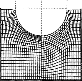
grangian displacement associated with deformation. Figure 1.8 compares the

mesh produced using the Lagrangian formulation (left side) with the mesh pro-

duced by the ALE formulation (right side) when modelling metal forging. The

Lagrangian mesh presents a high distortion, while the ALE is more regular and

presents low distortion.

The ALE formulation has two major drawbacks. Often the ALE formulation cannot

prevent the need for a complete re-meshing. The re-mapping of state variables is also

a drawback compared to the updated Lagrangian formulation. When the re-map is

performed inaccurately, the history of the material is not taken into account properly.

1.2.2 Modelling Chip Separation from the Workpiece

and Chip Segmentation

There are a number of numerical techniques to model chip separation from the rest of

the work material. The node-splitting technique is the oldest, where chip separation is

modelled by the separation of nodes of the mesh ahead of the tool cutting edge along

the predefined cutting line. This technique is usually used with the Lagrangian for-

mulation to simulate steady-state cutting. A number of separation criteria grouped as

geometrical and physical have been developed [28,

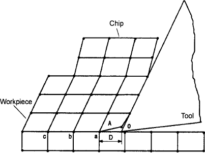
32−40]. According to the geo-

metrical criteria, the separation of two nodes occurs when the distance D between the

tool cutting edge (point O, in Figure 1.9) and the node immediately ahead (node a)

becomes less than a predefined critical value. According to the physical criteria, the

Figure 1.8. Comparison between a mesh produced by the Lagrangian formulation (left

side) and a mesh produced by the ALE formulation (right side)

16 V.P. Astakhov and J.C. Outeiro

separation of two nodes occurs when the value of a predefined physical parameter,

such as stress, strain or strain energy density, at node a or element A (Figure 1.9)

achieves a predefined critical value, selected depending upon the work material

properties and the cutting regime.

The physical criteria seem to be more adequate for modelling node splitting as

they are based on physical measurable properties of the work material. The prob-

lem, however, is in the selection of suitable representations of these properties. For

example, Chen and Black [38] argued that the critical strain energy density com-

monly used as a separation criterion is determined from a uniaxial tensile test and

thus cannot be considered as relevant in metal cutting.

1.2.3 Mesh Design

The first step in any finite element or finite boundary analysis includes dividing the

continuum or solution region into finite elementary regions (lines, areas or volumes)

called elements. This procedure to converting a continuous region into a discrete re-

gion is referred to as discretization, included in a large topic named as mesh design.

The problems related to mesh design are not restricting to the initial discretiza-

tion procedure. In metal cutting modelling, the common problem is related to the

element distortion during the simulations due to severe plastic deformation. The

distortion can cause a deterioration of the FE simulation in terms of convergence

rate and numerical errors, or cause the Jacobian determinant to become negative,

which makes further analysis impossible. It is often necessary to redefine the mesh

after some stages of deformation.

Several techniques are used to reduce the element distortion: re-meshing, smooth-

ing and refinement. These techniques include the generation of a completely new

finite element mesh out of the existing mesh, increasing the local element density

by reducing the local element size (Figure 1.10) and/or reallocating the individual

nodes to improve the local quality of the elements (Figure 1.11).

Figure 1.9. Separation of nodes based in the distance D between the tool cutting edge

(point O) and the node immediately ahead (node a)

Metal Cutting Mechanics, Finite Element Modelling 17

Figure 1.10. Increase local mesh density (refinement)

Figure 1.11. Reallocation of the nodes (smoothing)

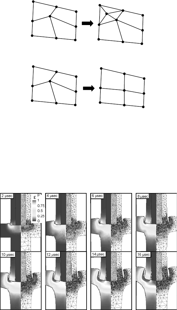
The discussed techniques are used in the so-called adaptive mesh procedure.

Adaptive mesh refers to a scheme for finite difference and finite element codes

wherein the size and distribution of the mesh is changed dynamically during the

simulations. In the regions of strong gradients of variables involved, a higher mesh

density is needed in order to decrease the solution errors. As these gradients are

not known a priori, the adaptive mesh generation procedure starts with a relatively

coarse primary mesh and, after obtaining the solution on this primary mesh, the

mesh density is increased for the strong gradients.

Figure 1.12. Example showing the concept of the adaptive mesh in modelling strong gradients

Davim J. Paulo (editor). Machining. Fundamentals and Recent Advances

Подождите немного. Документ загружается.