Bonchev D., Rouvray D.H. (editors) Complexity in Chemistry, Biology, and Ecology

Подождите немного. Документ загружается.

172 Chapter 4

vertices e

to be q

, the simple product of remaining degrees. If that is

not the value found, we can measure the difference by averaging through

all the edges in the graph, that is,





−









jk(e

− q

This sum measures the assortativeness of a network [20]. If it is positive,

high degree nodes tend to connect to other high degree nodes, whereas a

negative value describes the opposite, high degree nodes will preferentially

be neighbors of low degree ones.

To properly compare different networks, it is convenient to normalize

the sum by the maximum value attainable, so that the result is in the range

(−1, 1). The maximum value, in fact, is present when the joint distri-

bution e

is simply q

, that is, when nodes of a given degree just

connect to nodes of the same degree. It is easy to see that the result is



− [

]

which is the variance of the remaining degree distri-

bution, σ

. Hence, the normalized correlation function is

r =



jk(e

− q

). (4.1)

When calculating this value for an actual network with known values, we

can use the following formula [20],

r =

−1



−



−1



( j

+ k

)



−1





+ k



−



−1



( j

+ k

)



(4.2)

where j

, k

are the degrees of the vertices at the ends of the ith edge, with i

=1,...L. When we apply this measure to protein interaction networks, the

results are clear, protein networks are disassortative, that is, hubs connect

with high correlation to low degree nodes. The results for the three networks

in Figure 4.10 are, respectively, −0.1302, −0.1361 and −0.1397.

4.2. Correlation proﬁles

However, the assortativeness of a network gives just a global description

of the correlations in connectivity. If we want more detail in this type of

analysis, we have to turn to other techniques. One more time, measure-

ments will involve the comparison of the correlations of a given graph with

its randomized counterpart [21,22]. Since we are comparing degree corre-

lations, though, it is important in this case to create a random graph that

has the same degree distribution.

Graphs as Models of Large-Scale Biochemical Organization 173

This is achieved through a rewiring process, in which the degree dis-

tribution is preserved. If two edges are chosen at random that do not have

vertices in common, the simple exchange of their starting vertices will give

a graph with the same degree distribution but otherwise random. Iterating

this process as many times as twice the number of edges yields a reasonably

randomized graph, with preserved degree distribution. If we call P(k

, k

)

the probability of ﬁnding an edge connecting two nodes with degree k

and

, and P

, k

) the random equivalent, we can measure twothings, that is,

R(k

, k

) =

P(k

, k

)

, k

)

, (4.3)

whose deviation manifest the correlations, and

Z(k

, k

) =

P(k

, k

) − P

, k

)

, k

)

, (4.4)

quantifying the statistical signiﬁcance of R(k

, k

), or Z-score. The value

, k

) is the standard deviation of P

, k

) in an ensemble of random-

ized networks.

Theresults of this process are shownin Figure 4.11. The imagerepresents

a log-binned matrix in which black indicates a higher value, as the side bar

shows. This proﬁle reveals, with some more precision, the disassortative

nature of protein interaction networks.

1.0 3.2 10.0 31.6 100.0 316.2

1.0

3.2

10.0

31.6

100.0

316.2

0.00

0.25

0.50

0.75

1.00

1.25

1.0 3.2 10.0 31.6 100.0 316.2

1.0

3.2

10.0

31.6

100.0

316.2

−8.0

−6.0

−4.0

−2.0

0.0

2.0

4.0

6.0

8.0

10.0

12.0

Figure 4.11. (A) Correlation proﬁle of the protein interaction network, with the dataset

taken from [18]. The value R(k

, k

) is shown. (B) Same as A, but showing the Z-score,

Z(k

, k

174 Chapter 4

To ﬁnish our analysis of the proteome network, we can see its modu-

larity, which is something not apparent in the graph of Figure 4.9A, as we

mentioned in the introduction. In the last section we saw that hierarchical

clustering can give a clear picture of modularity lacking any good measure

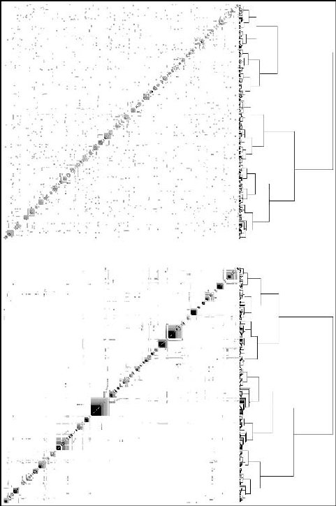
of it. A network such as the one shown in Figure 4.9A has a modularity

Figure 4.12. Bottom. Modular appearance of the network of Figure 9A. Top. The result of

applying the same algorithm to a random network of about the same size.

Graphs as Models of Large-Scale Biochemical Organization 175

that is revealed by the hierarchical clustering shown in Figure 4.12 (bot-

tom). The random network of Figure 4.9B is also displayed for comparison

(top).

4.3. Proteome model

Since we now know the structure of the proteome network, we can ask

ourselves how the proteome network emerged. In principle, we can try

to ﬁnd simple mechanisms that we know alter the relationship between

proteins in the genome and try to interpret them in terms of the rewiring

process that affects the protein interaction network. A simple mechanism

does, in fact, exist, and it gives a very plausible answer to the question of

the origin of the proteome network.

The genome grows mainly due to gene duplication. From time to time, a

gene is duplicated in the cell replication process that gives rise to a redun-

dant copy of a gene. After a while, mutations accumulate that make the two

copies diverge pushing their sequences apart, and as well the functionality

of the proteins they code for. The result is that most genes currently present

in the genome can be traced back to ancient duplications of other genes.

Since proteins are the product of genes, we can model gene duplication in

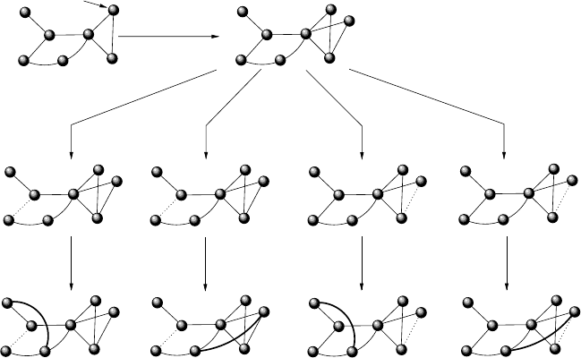
the way Figure 4.13 shows [23].

We start form a set m

of connected nodes, and at each time step we

perform the following operations

• One node of the graph is selected at random and duplicated

• The links emanating from the newly generated node are removed with

probability δ.

• New links (not previously present after the duplication step) are created

between the newnode and all any other node with probability α.Although

available data indicate that new interactions are likely to be formed pref-

erentially towards proteins with high degree here we do not consider this

constraint.

Step (i) implements gene duplication, in which both the original and the

replicated proteins retain the same structural properties and, consequently,

the same set of interactions. The rewiring steps (ii) and (iii) implement the

possible mutations of the replicated gene, which translate into the dele-

tion and addition of interactions with different proteins, respectively. The

process is repeated until N proteins have been obtained.

176 Chapter 4

αα α

NC C NC

(1)

(2)

(3)

Figure 4.13. Rules of proteome growth in the four possible scenarios. First, (1) duplication

occurs after randomly selecting a node (small arrow). Then (2) deletion of connections

occurs with probability δ. This event can be correlated (C) when the deleted links are con-

nected to the newly generated node or uncorrelated (NC), when all links are considered

for deletion. Finally (3) new connections are generated with probability α, again in a cor-

related or uncorrelated way. The time scales at which different events occur are known to

be very different: duplication takes place at a much slower rate, whereas rewiring is much

faster. Additionally, the speciﬁc rates at which each event occur might involve preferential

attachment to proteins of higher connectivity. All these variants can be included.

Another model uses very similar rules [24], but introduces some relevant

differences. Duplication is also followed by two probabilistic rules which

operate independently. The ﬁrst (ii) islink deletion. For each of the nodes p

linked to the two p

and its duplicate p



, we choose randomly one of the two

links ε

, ε



and remove it withprobability δ. Additionally, a newinteraction

connecting the two proteins (the parent and the duplicated) is introduced

with probability ρ. The last rule will naturally increase the number of

triangles in the system and thus provide a source of high clustering.

The rewiring process seems to be more appropriately deﬁned, since the

removal of one of the alternative links allows “conserving” the function

that was somehow present before the duplication event. In Sol´e’s model,

the whole set of links of the duplicated gene are preserved and loss of

Graphs as Models of Large-Scale Biochemical Organization 177

connections affects only the new copy. By using V´azquez’s approach, more

ﬂexibility is allowed and the interaction map is more likely to remain

connected. As deﬁned, it is important to note that duplicates will diverge

only to some extent: if duplication occurs in a gene with degree k

, only

δk

will be removed on average.

The two models collapse into a single mean ﬁeld description where the

average connectivity follows the dynamics

(

+ φ

(n, K

) − 2δK

)

, (4.5)

where φ = 2α(n − K

) in Sol´e’s model and φ = 2α(n − K

) = ρ in

V´azquez’s model. Actually, in previous work [23] it is shown that in order

to have convergence in the system towards a scale-free stationary distribu-

tion we need a very small rate of link addition (which is consistent with

observations). If we assume that α ∼ O(1/n) then a single link is added on

average each step and thus the two models are identical in the low-addition

limit. Speciﬁcally, if the graph is sparse, we have α(n − K

) ≈ ρ, which

results in a dynamical equation

2δ − 1

2ρ

(4.6)

which has an associated general solution

= e

−η(n)



2ρ



−η(n)

dn + C



(4.7)

where η(n) =



(2δ − 1)dn/n = (2δ − 1) ln n.

This gives

2ρ

2δ − 1



−

2ρ

2δ − 1



−(2δ−1)

(4.8)

if δ>δ

= 1/2, the previous system converges to a graph with a ﬁnite

average degree

∞

= lim

n→∞

2ρ

2δ − 1

(4.9)

Otherwise, the average connectivity will be K

∞

→∞. The critical re-

moval rate δc = 1/2 thus deﬁnes a phase transition separating a phase with

a highly-connected system (δ<δ

= 1/2) from a sparse phase (δ>δ

)

where a ﬁnite number of links will be observed. At this phase, the network

178 Chapter 4

becomes fragmented into many components. It is interesting to note that,

under the present conditions, the long-term behavior of the average connec-

tivity does not depend on the rate of link addition. What is really important

is that the rate of link addition and link removal are similar, so that k

can reach a stationary value. Moreover, it can be shown that although no

explicit preferential attachment is included here, the multiplicative nature

of the process (in which proteins having more links are more likely to have

them copied) actually leads to an effective preferential attachment [25].

We can test this prediction by studying the behavior of the model under

different rates of link deletion. In order to measure the impact of this rate on

network’s architecture, we use two different, but closely related measures:

(1) the normalized largestcomponent size S and (2) the average,normalized

component size





.IfC() = {

, 

,...,

} is the set of connected

components (subgraphs) of the proteome map, so that

 =

∞



i=1



(4.10)

and n

=|

| indicates their size (with



= N ), we deﬁne

S =

max{n

} (4.11)









i=1



(4.12)

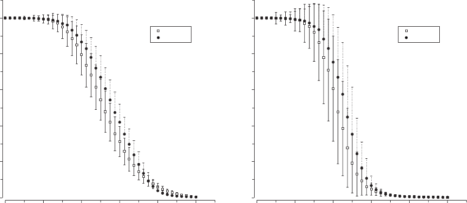
In Figure 4.14 we display the two measures against δ foraN= 10

protein network. Close to δ

we can appreciate a clear change. The two

phases are clearly identiﬁed, with the connected one showing S ≈1,





≈1

and the fragmented phase showing S ≈ 1/N,





≈ 1/N. In Figure 4.14

(left) we can see that S decreases slowly close to δ

, where only about

half of the nodes remain connected within the largest component. The

sharpness of the transition becomes much more obvious in Figure 4.14

(right). Here we clearly appreciate the impact of rewiring on network’s

structure, indicating that a large fraction of the overall network structure

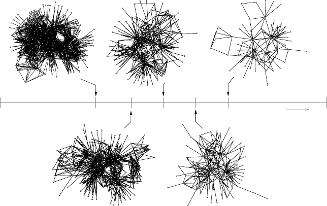
is formed by small, isolated components. In Figure 4.15 we can see some

examplesof the graphs generated (largestcomponents) obtained at different

rates of deletion.

0 0,2

0,4

0,6 0,8

0,0

0,2

0,4

0,6

0,8

1,0

Largest component size

Model A

Model B

0,0 0,2

0,4

0,6 0,8

1,0

0,0

0,2

0,4

0,6

0,8

1,0

Average component size

Model A

Model B

Figure 4.14. Phase transition in the genome growth models. Here

N = 10

and averages have been performed over R

= 10

replicas.

Here the size of the largest component and the average size are shown against the rate of link removal

δ. The predicted phase transition

occurs at

≈ 0.5. Due to the ﬁnite (small) size of our networks, the transition

appears to be less sharp than expected.

179

180 Chapter 4

0.6 0.70.50.40.30.0

1.0

Figure 4.15. The architecture of the proteome map, as generated by the simple model for

different values of the deletion rate δ. As predicted by the mathematical model, two well-

deﬁned phases are present. For the ﬁrst, when δ<δ

= 0.5, the protein map is highly

connected and most elements have links to others. Conversely, for δ>δ

, the graph is

fragmented into many components and many components have no links or belong to small

isolated subnets. Close to the transition domain, we have a sparse graph with the statistical

features displayed by the real proteome map. Such graph displays modular organization, in

spite of a complete lack of functionality in the deﬁnition of the model rules.

5. Gene Networks

The proteome network of last section demonstrates the importance of

models that try to capture essential ingredients in network evolution. We

have seen the networks implicit in protein structures, the networks that

these molecules form when interacting within the cell as numerous com-

plexes, but we are still lacking one important ingredient, and that is func-

tion. Although illuminating, previous analyses dealt only with topological

properties, which can describe cells only partially. If we really want to

understand cellular functioning, we must turn towards its function, and in

particular, to regulatory networks.

It is known since long ago that genes interact with one another. This

interaction is due to the fact that some proteins (transcription factors) can

Graphs as Models of Large-Scale Biochemical Organization 181

bind to DNA and alter transcription of other proteins, modulating their

concentrations. This regulation allows us to model a genome as a network:

each gene is mapped to a node, and regulatory interactions are mapped to

the edges between them. Since the existence of regulatory interaction from

gene a to b doesn’t necessarily imply also that b regulates a, we are in fact

considering a directed network.

To be able to model this kind of networks, we can simplify things by

considering a discretized version of a genome: although gene expression is

known to be continuous, we can disregard this and consider genes Boolean.

This approximation was pioneered by Kauffman more that 30 years ago

[26]. This type of analysis, although to some purposes too simple, has been

successful in models of genetic circuits [27,28]. In this kind of modeling, a

gene is just like a switch, which can be turned on or off, that is, expressed

or not expressed. The nodes in the network are then represented by a set of

Boolean variables {σ

, σ

,...,σ

}, which are, in fact, functions of discrete

time. To determine the value of each gene in the next time step, we will

use the values of the inputs of this gene, i.e., the values of the genes that

regulate it, and to combine the diverse values of the inputs of a gene, a

general function f

is assumed to operate. In general, then, the dynamics

of gene σ

(t + 1) = f

(σ

,σ

, ..., σ

), (5.1)

where k is the number of regulatory inputs of σ

. In the general case, and

without applying any explicit knowledge about the connectivityof real gene

networks or the combinations of values performed in real genes, we can

assume those to be random. First, the presence of an interaction between

gene i and j will depend on a certain probability, which is the deﬁnition

of a random graph, yielding a Poisson distribution for the number





incoming links. Second, to make functions random, for every combination

of values in the inputs, the value of the output will be 1 with probability

p and 0 with probability 1 − p. This leaves a control over the bias in the

function, but leaves it otherwise random. Summarizing, we have a discrete

dynamics over a random graph with random functions of Boolean values,

a Random Boolean Network (RBN).

Since Boolean networks are deterministic systems, whenever a network

reaches a state which has already been visited in a previous time-step, it

will enter in a cyclic trajectory. Due to this fact, the whole state space with

 = 2

conﬁgurations is nicely partitioned into these cycles and their