Bhadeshia H.K.D.H. Worked Examples in the Geometry of Crystals
Подождите немного. Документ загружается.

.
Worked examples in the
Geometry of Crystals
Second edition
H. K. D. H. Bhadeshia
Professor of Physical Metallurgy
University of Cambridge
Adjunct Professor of Computational Metallurgy
Graduate Institute of Ferrous Technology
POSTECH, South Korea
Fellow of Darwin College, Cambridge
i

Book 377
ISBN 0 904357 94 5
First edition published in 1987 by
The Institute of Metals The Institute of Metals
1 Carlton House Terrace and North American Publications Center
London SW1Y 5DB Old Post Road
Brookfield, VT 05036, USA
c
! THE INSTITUTE OF METALS 1987
ALL RIGHTS RESERVED
British Library Cataloguing in Publication Data
Bhadeshia, H. K. D. H.
Worked examples in the geometry of crystals.
1. Crystallography, Mathematical —–
Problems, exercises, etc.
I. Title
548’.1 QD911
ISBN 0–904357–94–5
COVER ILLUSTRATION
shows a net–like sub–grain boundary
in annealed bainite, ×150, 000.
Photograph by courtesy of J. R. Yang
Compiled from original typesetting and
illustrations provided by the author
SECOND EDITION, published 2001, updated 2006
Published electronically with permission
from the Institute of Materials
1 Carlton House Terrace
London SW1Y 5DB
ii
Preface
First Edition
A large part of crystallography deals with the way in which atoms are arranged in single crys-
tals. On the other hand, a knowledge of the relationships between crystals in a polycrystalline
material can be fascinating from the point of view of materials science. It is this aspect of
crystallography which is the subject of this monograph. The monograph is aimed at both
undergraduates and graduate students and assumes only an elementary knowledge of crystal-
lography. Although use is made of vector and matrix algebra, readers not familiar with these
methods should not be at a disadvantage after studying appendix 1. In fact, the mathematics
necessary for a good grasp of the subject is not very advanced but the concepts involved can
be difficult to absorb. It is for this reason that the book is based on worked examples, which
are intended to make the ideas less abstract.
Due to its wide–ranging applications, the subject has developed with many different schemes
for notation and this can be confusing to the novice. The extended notation used throughout
this text was introduced first by Mackenzie and Bowles; I believe that this is a clear and
unambiguous scheme which is particularly powerful in distinguishing between representations
of deformations and axis transformations.
The monograph begins with an introduction to the range of topics that can be handled using
the concepts developed in detail in later chapters. The introduction also serves to familiarise
the reader with the notation used. The other chapters cover orientation relationships, aspects
of deformation, martensitic transformations and interfaces.
In preparing this book, I have benefited from the support of Professors R. W. K. Honeycombe,
Professor D. Hull, Dr F. B. Pickering and Professor J. Wood. I am especially grateful to
Professor J. W. Christian and Professor J. F. Knott for their detailed comments on the text,
and to many students who have over the years helped clarify my understanding of the subject.
It is a pleasure to acknowledge the unfailing support of my family.
April 1986
Second Edition
I am delighted to be able to publish this revised edition in electronic form for free access. It is
a pleasure to acknowledge valuable comments by Steven Vercammen.
January 2001, updated July 2008
iii
Contents
INTRODUCTION . . . . . . . . . . . . . . . . . . . . . . . . . . . . . . . . . . . . . . . . . . . . . . . . . . . . . . . . . . . . . . . . . . . . . . . 1
Definition of a Basis . . . . . . . . . . . . . . . . . . . . . . . . . . . . . . . . . . . . . . . . . . . . . . . . . . . . . . . . . . . . . . . . . . . . . .2
Co-ordinate transformations . . . . . . . . . . . . . . . . . . . . . . . . . . . . . . . . . . . . . . . . . . . . . . . . . . . . . . . . . . . . . . 3
The reciprocal basis . . . . . . . . . . . . . . . . . . . . . . . . . . . . . . . . . . . . . . . . . . . . . . . . . . . . . . . . . . . . . . . . . . . . . . 5
Homogeneous deformations . . . . . . . . . . . . . . . . . . . . . . . . . . . . . . . . . . . . . . . . . . . . . . . . . . . . . . . . . . . . . . . 6
Interfaces . . . . . . . . . . . . . . . . . . . . . . . . . . . . . . . . . . . . . . . . . . . . . . . . . . . . . . . . . . . . . . . . . . . . . . . . . . . . . . . . 9
ORIENTATION RELATIONS . . . . . . . . . . . . . . . . . . . . . . . . . . . . . . . . . . . . . . . . . . . . . . . . . . . . . . . . . . 12
Cementite in Steels . . . . . . . . . . . . . . . . . . . . . . . . . . . . . . . . . . . . . . . . . . . . . . . . . . . . . . . . . . . . . . . . . . . . . 13
Relations between FCC and BCC crystals . . . . . . . . . . . . . . . . . . . . . . . . . . . . . . . . . . . . . . . . . . . . . . . 16
Orientation relations between grains of identical structure . . . . . . . . . . . . . . . . . . . . . . . . . . . . . . . .19
The metric . . . . . . . . . . . . . . . . . . . . . . . . . . . . . . . . . . . . . . . . . . . . . . . . . . . . . . . . . . . . . . . . . . . . . . . . . . . . . .22
More about the vector cross product . . . . . . . . . . . . . . . . . . . . . . . . . . . . . . . . . . . . . . . . . . . . . . . . . . . . 24
SLIP, TWINNING AND OTHER INVARIANT-PLANE STRAINS . . . . . . . . . . . . . . . . . . . . . . 25
Deformation twins . . . . . . . . . . . . . . . . . . . . . . . . . . . . . . . . . . . . . . . . . . . . . . . . . . . . . . . . . . . . . . . . . . . . . . 31
The concept of a Correspondence matrix . . . . . . . . . . . . . . . . . . . . . . . . . . . . . . . . . . . . . . . . . . . . . . . . 35
Stepped interfaces . . . . . . . . . . . . . . . . . . . . . . . . . . . . . . . . . . . . . . . . . . . . . . . . . . . . . . . . . . . . . . . . . . . . . . .34
Eigenvectors and eigenvalues . . . . . . . . . . . . . . . . . . . . . . . . . . . . . . . . . . . . . . . . . . . . . . . . . . . . . . . . . . . . 39
Stretch and rotation . . . . . . . . . . . . . . . . . . . . . . . . . . . . . . . . . . . . . . . . . . . . . . . . . . . . . . . . . . . . . . . . . . . . 41
Conjugate of an invariant-plane strain . . . . . . . . . . . . . . . . . . . . . . . . . . . . . . . . . . . . . . . . . . . . . . . . . . . 48
MARTENSITIC TRANSFORMATIONS . . . . . . . . . . . . . . . . . . . . . . . . . . . . . . . . . . . . . . . . . . . . . . . . 51
The diffusionless nature of martensitic transformations . . . . . . . . . . . . . . . . . . . . . . . . . . . . . . . . . . .51
The interface between the parent and product phases . . . . . . . . . . . . . . . . . . . . . . . . . . . . . . . . . . . . 51
Orientation relationships . . . . . . . . . . . . . . . . . . . . . . . . . . . . . . . . . . . . . . . . . . . . . . . . . . . . . . . . . . . . . . . . 54
The shape deformation due to martensitic transformation . . . . . . . . . . . . . . . . . . . . . . . . . . . . . . . .55
The phenomenological theory of martensite crystallography . . . . . . . . . . . . . . . . . . . . . . . . . . . . . . 57
INTERFACES IN CRYSTALLINE SOLIDS . . . . . . . . . . . . . . . . . . . . . . . . . . . . . . . . . . . . . . . . . . . . . 70
Symmetrical tilt boundary . . . . . . . . . . . . . . . . . . . . . . . . . . . . . . . . . . . . . . . . . . . . . . . . . . . . . . . . . . . . . . 73
The interface between alpha and beta brass . . . . . . . . . . . . . . . . . . . . . . . . . . . . . . . . . . . . . . . . . . . . . .75
Coincidence site lattices . . . . . . . . . . . . . . . . . . . . . . . . . . . . . . . . . . . . . . . . . . . . . . . . . . . . . . . . . . . . . . . . . 76
Multitude of axis-angle pair representations . . . . . . . . . . . . . . . . . . . . . . . . . . . . . . . . . . . . . . . . . . . . . .79
The O-lattice . . . . . . . . . . . . . . . . . . . . . . . . . . . . . . . . . . . . . . . . . . . . . . . . . . . . . . . . . . . . . . . . . . . . . . . . . . . 82
Secondary dislocations . . . . . . . . . . . . . . . . . . . . . . . . . . . . . . . . . . . . . . . . . . . . . . . . . . . . . . . . . . . . . . . . . . 85
The DSC lattice . . . . . . . . . . . . . . . . . . . . . . . . . . . . . . . . . . . . . . . . . . . . . . . . . . . . . . . . . . . . . . . . . . . . . . . . 86
Some difficulties associated with interface theory . . . . . . . . . . . . . . . . . . . . . . . . . . . . . . . . . . . . . . . . .89
APPENDIX 1: VECTORS AND MATRICES . . . . . . . . . . . . . . . . . . . . . . . . . . . . . . . . . . . . . . . . . . . 91
APPENDIX 2: TRANSFORMATION TEXTURE . . . . . . . . . . . . . . . . . . . . . . . . . . . . . . . . . . . . . . .96
APPENDIX 3: TOPOLOGY OF GRAIN DEFORMATION . . . . . . . . . . . . . . . . . . . . . . . . . . . . 100
REFERENCES . . . . . . . . . . . . . . . . . . . . . . . . . . . . . . . . . . . . . . . . . . . . . . . . . . . . . . . . . . . . . . . . . . . . . . . . 105
iv
1 Introduction
Crystallographic analysis, as applied in materials science, can be classified into two main
subjects; the first of these has been established ever since it was realised that metals have a
crystalline character, and is concerned with the clear description and classification of atomic
arrangements. X–ray and electron diffraction methods combined with other structure sensitive
physical techniques have been utilised to study the crystalline state, and the information
obtained has long formed the basis of investigations on the role of the discrete lattice in
influencing the behaviour of commonly used engineering materials.
The second aspect, which is the subject of this monograph, is more recent and took off in earnest
when it was noticed that accurate experimental data on martensitic transformations showed
many apparent inconsistencies. Matrix methods were used in resolving these difficulties, and
led to the formulation of the phenomenological theory of martensite
1,2
. Similar methods have
since widely been applied in metallurgy; the nature of shape changes accompanying displacive
transformations and the interpretation of interface structure are two examples. Despite the
apparent diversity of applications, there is a common theme in the various theories, and it is
this which makes it possible to cover a variety of topics in this monograph.
Throughout this monograph, every attempt has been made to keep the mathematical content
to a minimum and in as simple a form as the subject allows; the student need only have
an elementary appreciation of matrices and of vector algebra. Appendix 1 provides a brief
revision of these aspects, together with references to some standard texts available for further
consultation.
The purpose of this introductory chapter is to indicate the range of topics that can be tackled
using the crystallographic methods, while at the same time familiarising the reader with vital
notation; many of the concepts introduced are covered in more detail in the chapters that follow.
It is planned to introduce the subject with reference to the martensite transformation in steels,
which not only provides a good example of the application of crystallographic methods, but
which is a transformation of major practical importance.
At temperatures between 1185 K and 1655 K, pure iron exists as a face–centred cubic (FCC)
arrangement of iron atoms. Unlike other FCC metals, lowering the temperature leads to the
formation of a body–centred cubic (BCC) allotrope of iron. This change in crystal structure
can occur in at least two different ways. Given sufficient atomic mobility, the FCC lattice can
undergo complete reconstruction into the BCC form, with considerable unco–ordinated diffu-
sive mixing–up of atoms at the transformation interface. On the other hand, if the FCC phase
is rapidly cooled to a very low temperature, well below 1185 K, there may not be enough time
or atomic mobility to facilitate diffusional transformation. The driving force for transformation
1
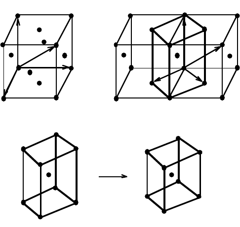
(a)
BAIN
STRAIN
(c )
Body-centered
tetragonal
austenite
(d )
Body-centered
cubic martensite
a
a
a
1
2
3
b
3
b
1
b
2
u u
(b )
INTRODUCTION
nevertheless increases with undercooling below 1185 K, and the diffusionless formation of BCC
martensite eventually occurs, by a displacive or “shear” mechanism, involving the systematic
and co–ordinated transfer of atoms across the interface. The formation of this BCC martensite
is indicated by a very special change in the shape of the austenite (γ) crystal, a change of shape
which is beyond that expected just on the basis of a volume change effect. The nature of this
shape change will be discussed later in the text, but for the present it is taken to imply that the
transformation from austenite to ferrite occurs by some kind of a deformation of the austenite
lattice. It was E. C. Bain
3
who in 1924 introduced the concept that the structural change from
austenite to martensite might occur by a homogeneous deformation of the austenite lattice, by
some kind of an upsetting process, the so–called Bain Strain.
Definition of a Basis
Before attempting to deduce the Bain Strain, we must establish a method of describing the
austenite lattice. Fig. 1a shows the FCC unit cell of austenite, with a vector u drawn along the
cube diagonal. To specify the direction and magnitude of this vector, and to relate it to other
vectors, it is necessary to have a reference set of co–ordinates. A convenient reference frame
would be formed by the three right–handed orthogonal vectors a
1
, a
2
and a
3
, which lie along
the unit cell edges, each of magnitude a
γ
, the lattice parameter of the austenite. The term
orthogonal implies a set of mutually perpendicular vectors, each of which can be of arbitrary
magnitude; if these vectors are mutually perpendicular and of unit magnitude, they are called
orthonormal.
Fig. 1:
(a) Conventional FCC unit cell. (b) Relation between FCC and BCT
cells of austenite. (c) BCT cell of austenite. (d) Bain Strain deforming the
BCT austenite lattice into a BCC martensite lattice.
2

The set of vectors a
i
(i = 1, 2, 3) are called the basis vectors, and the basis itself may be
identified by a basis symbol, ‘A’ in this instance.
The vector u can then be written as a linear combination of the basis vectors:
u = u
1
a
1
+ u
2
a
2
+ u
3
a
3
,
where u
1
, u
2
and u
3
are its components, when u is referred to the basis A. These components
can conveniently be written as a single–row matrix (u
1
u
2
u
3
) or as a single–column matrix:
u
1
u
2
u
3
This column representation can conveniently be written using square brackets as: [u
1
u
2
u
3
].
It follows from this that the matrix representation of the vector u (Fig. 1a), with respect to
the basis A is
(u; A) = (u
1
u
2
u
3
) = (1 1 1)
where u is represented as a row vector. u can alternatively be represented as a column vector
[A; u] = [u
1
u
2
u
3
] = [1 1 1]
The row matrix (u;A) is the transpose of the column matrix [A;u], and vice versa. The
positioning of the basis symbol in each representation is important, as will be seen later. The
notation, which is due to Mackenzie and Bowles
2
, is particularly good in avoiding confusion
between bases.
Co–ordinate Transformations
From Fig. 1a, it is evident that the choice of basis vectors a
i
is arbitrary though convenient;
Fig. 1b illustrates an alternative basis, a body–centred tetragonal (BCT) unit cell describing
the same austenite lattice. We label this as basis ‘B’, consisting of basis vectors b
1
, b
2
and b
3
which define the BCT unit cell. It is obvious that [B; u] = [0 2 1], compared with [A; u] = [1 1 1].
The following vector equations illustrate the relationships between the basis vectors of A and
those of B (Fig. 1):
a
1
= 1b
1
+ 1b
2
+ 0b
3
a
2
= 1b
1
+ 1b
2
+ 0b
3
a
3
= 0b
1
+ 0b
2
+ 1b
3
These equations can also be presented in matrix form as follows:
(a
1
a
2
a
3
) = (b
1
b
2
b
3
) ×
1
1 0
1 1 0
0 0 1
(1)
This 3×3 matrix representing the co–ordinate transformation is denoted (B J A) and transforms
the components of vectors referred to the A basis to those referred to the B basis. The first
column of (B J A) represents the components of the basis vector a
1
, with respect to the basis
B, and so on.
3
0 1 0
1 0 0
1 0 0
0 1 0
A
B
B
A
4 5 °
INTRODUCTION
The components of a vector u can now be transformed between bases using the matrix (B J A)
as follows:
[B; u] = (B J A)[A; u] (2a)
Notice the juxtapositioning of like basis symbols. If (A J’ B) is the transpose of (B J A), then
equation 2a can be rewritten as
(u; B) = (u; A)(A J
!
B) (2b)
Writing (A J B) as the inverse of (B J A), we obtain:
[A; u] = (A J B)[B; u] (2c)
and
(u; A) = (u; B)(B J
!
A) (2d)
It has been emphasised that each column of (B J A) represents the components of a basis
vector of A with respect to the basis B (i.e. a
1
= J
11
b
1
+ J
21
b
2
+ J
31
b
3
etc.). This procedure
is also adopted in (for example) Refs. 4,5. Some texts use the convention that each row of
(B J A) serves this function (i.e. a
1
= J
11
b
1
+ J
12
b
2
+ J
13
b
3
etc.). There are others where a
mixture of both methods is used – the reader should be aware of this problem.
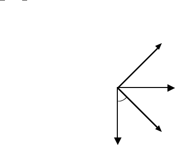
Example 1: Co–ordinate transformations
Two adjacent grains of austenite are represented by bases ‘A’ and ‘B’ respectively. The base
vectors a
i
of A and b
i
of B respectively define the FCC unit cells of the austenite grains
concerned. The lattice parameter of the austenite is a
γ
so that |a
i
| = |b
i
| = a
γ
. The grains are
orientated such that [0 0 1]
A
# [0 0 1]
B
, and [1 0 0]
B
makes an angle of 45
◦
with both [1 0 0]
A
and [0 1 0]
A
. Prove that if u is a vector such that its components in crystal A are given by
[A; u] = [
√
2 2
√
2 0], then in the basis B, [B; u] = [3 1 0]. Show that the magnitude of u (i.e.
|u|) does not depend on the choice of the basis.
Fig. 2:
Diagram illustrating the relation between the bases A and B.
Referring to Fig. 2, and recalling that the matrix (B J A) consists of three columns, each
column being the components of one of the basis vectors of A, with respect to B, we have
[B; a
1
] = [ cos 45 −sin 45 0]
[B; a
2
] = [ sin 45 cos 45 0]
[B; a
3
] = [ 0 0 1]
and (B J A) =
cos 45 sin 45 0
−sin 45 cos 45 0
0 0 1
4

From equation 2a, [B; u] = (B J A)[A; u], and on substituting for [A; u] = [
√
2 2
√
2 0], we get
[B; u] = [3 1 0]. Both the bases A and B are orthogonal so that the magnitude of u can be
obtained using the Pythagoras theorem. Hence, choosing components referred to the basis B,
we get:
|u|
2
= (3|b
1
|)
2
+ (|b
2
|)
2
= 10a
2
γ
With respect to basis A,
|u|
2
= (
√
2|a
1
|)
2
+ (2
√
2|a
2
|)
2
= 10a
2
γ
Hence, |u| is invariant to the co–ordinate transformation. This is a general result, since a
vector is a physical entity, whose magnitude and direction clearly cannot depend on the choice
of a reference frame, a choice which is after all, arbitrary.
We note that the components of (B J A) are the cosines of angles between b
i
and a
j
and
that (A J
!
B) = (A J B)
−1
; a matrix with these properties is described as orthogonal (see
appendix). An orthogonal matrix represents an axis transformation between like orthogonal
bases.
The Reciprocal Basis
The reciprocal lattice that is so familiar to crystallographers also constitutes a special co-
ordinate system, designed originally to simplify the study of diffraction phenomena. If we
consider a lattice, represented by a basis symbol A and an arbitrary set of basis vectors a
1
, a
2
and a
3
, then the corresponding reciprocal basis A
∗
has basis vectors a
∗
1
, a
∗
2
and a
∗
3
, defined by
the following equations:
a
∗
1
= (a
2
∧ a
3
)/(a
1
.a
2
∧ a
3
) (3a)
a
∗
2
= (a
3
∧ a
1
)/(a
1
.a
2
∧ a
3
) (3b)
a
∗
3
= (a
1
∧ a
2
)/(a
1
.a
2
∧ a
3
) (3c)
In equation 3a, the term (a
1
.a
2
∧a
3
) represents the volume of the unit cell formed by a
i
, while
the magnitude of the vector (a
2
∧a
3
) represents the area of the (1 0 0)
A
plane (see appendix).
Since (a
2
∧ a
3
) points along the normal to the (1 0 0)
A
plane, it follows that a
∗
1
also points
along the normal to (1 0 0)
A
and that its magnitude |a
∗
1
| is the reciprocal of the spacing of the
(1 0 0)
A
planes (Fig. 3).
The reciprocal lattice is useful in crystallography because it has this property; the components
of any vector referred to the reciprocal basis represent the Miller indices of a plane whose normal
is along that vector, with the spacing of the plane given by the inverse of the magnitude of
that vector. For example, the vector (u; A
∗
) = (1 2 3) is normal to planes with Miller indices
(1 2 3) and interplanar spacing 1/|u|. Throughout this text, the presence of an asterix indicates
reference to the reciprocal basis. Wherever possible, plane normals will be written as row
vectors, and directions as column vectors.
We see from equation 3 that
a
i
.a
∗
j
= 1 when i = j, and a
i
.a
∗
j
= 0 when i '= j
or in other words,
a
i
.a
∗
j
= δ
ij
(4a)
5
a
a
a
a
1
3
2
1
*
1
O
R
A
P
Q
INTRODUCTION
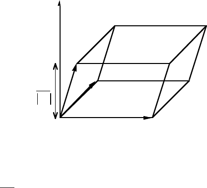
Fig. 3:
The relationship between a
∗
1
and a
i
. The vector a
∗
1
lies along the
direction OA
and the volume of the parallelepiped formed by the basis vectors
a
i
is given by a
1
.a
2
∧ a
3
, the area OPQR being equal to |a
2
∧ a
3
|.
δ
ij
is the Kronecker delta, which has a value of unity when i = j and is zero when i '= j (see
appendix).
Emphasising the fact that the reciprocal lattice is really just another convenient co–ordinate
system, a vector u can be identified by its components [A; u] = [u
1
u
2
u
3
] in the direct lattice
or (u; A
∗
) = (u
∗
1
u
∗
2
u
∗
3
) in the reciprocal lattice. The components are defined as usual, by the
equations:
u = u
1
a
1
+ u
2
a
2
+ u
3
a
3
(4b)
u = u
∗
1
a
∗
1
+ u
∗
2
a
∗
2
+ u
∗
3
a
∗
3
(4c)
The magnitude of u is given by
|u|
2
= u.u
= (u
1
a
1
+ u
2
a
2
+ u
3
a
3
).(u
∗
1
a
∗
1
+ u
∗
2
a
∗
2
+ u
∗
3
a
∗
3
)
Using equation 4a, it is evident that
|u|
2
= (u
1
u
∗
1
+ u
2
u
∗
2
+ u
3
u
∗
3
)
= (u; A
∗
)[A; u].
(4d)
This is an important result, since it gives a new interpretation to the scalar, or “dot” product
between any two vectors u and v since
u.v = (u; A
∗
)[A; v] = (v; A
∗
)[A; u] (4e)
Homogeneous Deformations
We can now return to the question of martensite, and how a homogeneous deformation might
transform the austenite lattice (parameter a
γ
) to a BCC martensite (parameter a
α
). Referring
to Fig. 1, the basis ‘A’ is defined by the basis vectors a
i
, each of magnitude a
γ
, and basis
6