Bednorz W. (ed.) Advances in Greedy Algorithms
Подождите немного. Документ загружается.


Provably-Efficient Online Adaptive Scheduling of Parallel Jobs Based on Simple Greedy Rules
441
number of nodes on the longest chain of the precedence dependencies. The release time r(J
i
)
of the job J
i
is the time at which J
i
becomes first available for processing. Each job is handled
by a dedicated thread scheduler, which operates in an online manner, oblivious to the future
characteristics of the dynamically unfolding DAG.
The job scheduler and the thread schedulers interact as follows. The job scheduler may
reallocate processors between scheduling quanta. Between quantum q - 1 and quantum q,
the thread scheduler of a given job J
i
determines the job's desire d(J
i
, q), which is the number
of processors J
i
wants for quantum q. Based on the desire of all running jobs, the job
scheduler follows its processor-allocation policy to determine the allotment a (J
i
, q) of the job
with the constraint that a (J
i
, q) ≤ d(J
i
, q). Once a job is allotted its processors, the allotment
does not change during the quantum.
A schedule X = (, π) of a job set
is defined as two mappings : ∪ V
i
→ {1, 2, … ,1},
and π : ∪
V
i
→ {1, 2, … , P}, which map the vertices of the jobs in the job set to the set
of time steps, and the set of processors on the machine respectively. A valid mapping must
preserve the precedence relationship of each job. For any two vertices u, v ∈ V
i
of the job J
i
, if
u ≺ v, then (u) < (v), i.e. the vertex u must be executed before the vertex v. A valid
mapping must also ensure that one processor can only be assigned to one job at any given
time. For any two vertices u and v, both (u) = (v) and π(u) = π(v) are true iff u = v.
Our scheduler uses makespan and mean response time as the performance measurement.
Definition 1 The makespan of a given job set
is the time taken to complete all the jobs in
, i.e. T( ) = max T(J
i
), where T(J
i
) denotes the completion time of job J
i
.
Definition 2 The response time of a job J
i
is T(J
i
) - r(J
i
), which is the duration between its
release time r(J
i
) and the completion time T(J
i
). The total response time of a job set is given
by R(
) = Σ (T(J
i
) - r(J
i
)) and the mean response time is ( ) = R( )/
.
The goal of the chapter is to show that our scheduler optimizes the makespan and mean
response time, and we use competitive analysis as a tool to evaluate and compare the
scheduling algorithm. The competitive analysis of an online scheduling algorithm is to
compare the algorithm against an optimal clairvoyant algorithm. Let T*( ) denote the
makespan of an arbitrary jobset
scheduled by an optimal scheduler, and T( ) denote the
makespan produced by an algorithm A for the job set . A deterministic algorithm A is said
to be c-competitive if there exists a constant b such that T(
) ≤ c ⋅ T*( ) + b holds for the
schedule of any job set. We will show that our algorithm is c-competitive in terms of the
makespan, where c is a small constant. Similarly, for the mean response time, we will show
that our algorithm is also constant-competitive for any batched jobs.
3. Algorithms
This section presents the job scheduler - RAD, and overviews the thread scheduler - A-
GREEDY [1].
RAD Job Scheduler
The job scheduler RAD unifies the space-sharing job scheduling algorithm DEQ [35, 27]
with the time-sharing RR algorithm. When the number of jobs is greater than the number of
processors, GRAD schedules the jobs in a batched, round-robin fashion, which allocates one
processor to each job with an equal share of time. When the number of jobs is not more than
the number of processors, GRAD uses DEQ as the job scheduler. DEQ gives each job an
equal share of spatial allotments unless the job requests for less.
Advances in Greedy Algorithms
442
When a batch of jobs are scheduled in the round-robin fashion, RAD maintains a queue of
jobs. At the beginning of each quantum, if there are more than P jobs, it pops P jobs from the
top of the queue, and allots one processor to each of them during the quantum. At the end of
the quantum, RAD pushes the P jobs back to the bottom of the queue if they are
uncompleted. The new jobs can be put into the queue once they are released.
DEQ attempts to give each job a fair share of processors. If a job requires less than its fair
share, however, DEQ distributes the extra processors to the other jobs. More precisely, upon
receiving the desires {d(J
i
, q)} from the thread schedulers of all jobs J
i
∈ , DEQ executes the
following processor-allocation algorithm:
1. Set n =
. If n = 0, return.
2. If the desire of every job J
i
∈ satisfies d(J
i
, q) ≥ P/n, assign each job a (J
i
, q) = P/n
processors.
3. Otherwise, let
’ = {J
i
∈ : d(J
i
, q) < P/n}. Assign a (J
i
, q) = d(J
i
, q) processors to each J
i
∈
’. Update = -
’, and P = P - Σ
’
d(J
i
, q). Go to Step 1.
Note that, at any quantum where the number of jobs is equal to the number of processors,
DEQ and RR give exactly the same processor allotment, and allocate each of P jobs with one
processor.
Adaptive Greedy Thread Scheduler
A-GREEDY [1] is an adaptive greedy thread scheduler with parallelism feedback. Between
quanta, it estimates its job's desire, and requests processors from the job scheduler. During
the quantum, it schedules the ready threads of the job onto the allotted processors greedily
[15, 5]. If there are more than a (J
i
, q) ready threads, A-GREEDY schedules any a (J
i
, q) of
them. Otherwise, it schedules all of them.
A- GREEDY's desire-estimation algorithm is parameterized in terms of a utilization parameter
> 0 and a responsiveness parameter ρ > 1, both of which can be adjusted for different levels of
guarantees for waste and completion time.
Before each quantum, A- GREEDY y for a job J
i
∈ provides parallelism feedback to the job
scheduler based on the J
i
’s history of utilization in the previous quantum. A- GREEDY
classifies quanta as “satisfied” versus “deprived” and “eficient” versus “inefficient.” A
quantum q is satisfied if a (J
i
, q) = d(J
i
, q), in which case J
i
’s allotment is equal to its desire.
Otherwise, the quantum is deprived.
1
The quantum q is efficient if A- GREEDY utilizes no less
than a fraction of the total allotted processor cycles during the quantum, where is the
utilization parameter. Otherwise, the quantum is inefficient. Under the four-way
classification, however, A- GREEDY only uses three: inefficient, efficient-and-satisfied, and
efficient-and-deprived.
Using this three-way classification and the job's desire for the previous quantum, A-
GREEDY computes the desire for the next quantum as follows:
• If quantum q - 1 was inefficient, decrease the desire, setting d(J
i
, q) = d(J
i
, q - 1)=½, where
ρ is the responsiveness parameter.
• If quantum q - 1 was efficient-and-satisfied, increase the desire, setting d(J
i
, q) = ρd(J
i
, q - 1).
• If quantum q - 1 was efficient-and-deprived, keep desire unchanged, setting d(J
i
, q) =
d(J
i
, q - 1).
1
We can extend the classification of “satisfied” versus “deprived” from quanta to time
steps. A job J
i
is satisfied (or deprived) at step t ∈ [L ⋅ q,L ⋅ q + 1, .. ,L(q + 1) - 1] if J
i
is satisfied
(resp. deprived) at the quantum q.
Provably-Efficient Online Adaptive Scheduling of Parallel Jobs Based on Simple Greedy Rules
443
4. Makespan
This section shows that GRAD is c-competitive with respect to makespan, where c denotes a
constant. The exact value of c is related to the choice of A-GREEDY's utilization and
responsiveness parameter, as will be explained shortly.
We first review the lower bounds of makespan. Given a job set
and P processors, lower
bounds on the makespan of any job scheduler can be obtained based on release time, work,
and span. Recall that, for a job J
i
∈ , the quantities r(J
i
), T
1
(J
i
), and T
∞
(J
i
) represent the
release time, work, and span of J
i
, respectively. Let T* ( ) denote the makespan produced
by an optimal scheduler on a job set on P processors. Let T
1
( ) = Σ T
1
(J
i
) denote the
total work of the job set. The following two inequalities give two lower bounds on the
makespan [6]:
(1)
(2)
To facilitate the analysis, we state a lemma from [1] that bounds the satisfied steps and the
waste of a single job scheduled by A-GREEDY. Recall that, the parameter ρ > 1 denotes A-
GREEDY's responsiveness parameter, > 0 its utilization parameter, and L the quantum
length.
Lemma 1 [1] For a job J
i
with work T
1
(J
i
) and span T
∞
(J
i
) on a machine with P processors,
A- GREEDY produces at most 2T
∞
(J
i
)/(1 - )+Llog
ρ
P +L satisfied steps, and it wastes at most
(1+ρ - )T
1
(J
i
) / processor cycles in the course of the computation. □
The following theorem analyzes the makespan of a job set scheduled by GRAD.
Theorem 2 Let ρ denote A-GREEDY's responsiveness parameter, its utilization parameter, and L
the quantum length. Then, GRAD completes a job set
on P processors in
(3)
time steps.
Proof. Suppose job J
k
is the last job completed among the jobs in . Let S(J
k
) denote the set of
satisfied steps for J
k
, and D(J
k
) denote its set of deprived steps. The job J
k
is scheduled to start
its execution at the beginning of the quantum q where Lq < r(J
k
) ≤ L(q + 1), which is the
quantum immediately after J
k
's release. Therefore, we have T( ) ≤ r(J
k
) + L + │S(J
k
)│ +
│D(J
k
)│. We now bound │S(J
k
)│ and │D(J
k
)│ respectively.
From Lemma 1, we know that the number of satisfied steps attributed to J
k
is at most
│S(J
k
)│≤ 2T
∞
(J
k
)/(1 - ) + Llog
ρ
P + L.
We now bound the total number of deprived steps D(J
k
) of job J
k
. For each step t ∈ D(J
k
),
GRAD applies either DEQ or RR as job scheduler. RR always allots all processors to jobs. By
definition, DEQ must have allotted all processors to jobs whenever J
k
is deprived.
Thus, the total allotment on such a step t is always equal to the total number of
processors P. Moreover, the total allotment of
over J
k
's deprived steps D(J
k
) is a
(
,D(J
k
)) = Σ Σ
a (J
i
, t) = P│D(J
k
)│. Since any allotted processor is either working
productively or wasted, the total allotment for any job J
i
is bounded by the sum of its total
Advances in Greedy Algorithms
444
work T
1
(J
i
) and total waste w(J
i
). By Lemma 1, the waste for the job J
i
is at most (ρ - + 1)/
times of its work. Thus, the total number of allotted processor cycles for job J
i
is at most T
1
(J
i
)
+ w(J
i
) ≤ (ρ + 1)T
1
(J
i
) /. The total number of allotted processor cycles for all jobs is at most
Σ
(ρ + 1)T
1
(J
i
) / = ((ρ + 1)/)T
1
( ). Given a ( ,D(J
k
)) ≤((ρ + 1)/)T
1
( ) and
a ( ,D(J
k
)) = P
│D(J
k
)│, we have │D(J
k
)│ ≤
.
Therefore, we can get
□
Since both T
1
( ) =P and max {T
∞
(J
i
) + r(J
i
)} are lower bounds of T*( ), we obtain the
following corollary.
Corollary 3 GRAD completes a job set
in
time steps, where T*( ) denotes the makespan of produced by an optimal clairvoyant scheduler. □
Since both the quantum length L and the processor number P are independent variables
with respect to any job set , Corollary 3 shows that GRAD is O(1)-competitive with respect
to makespan.
To better interpret the bound, let's substitute ρ = 1.2 and = 0.6, we have T(
) ≤ 8.67T*( ) +
Llg P/ lg 1.2 + 2L. Since both the quantum length L and the processor number P are
independent variables with respect to any job set
, GRAD is 8.67-competitive given ρ = 1.2
and = 0.6.
When = 0.5 and ρ approaches 1, the competitiveness ratio (ρ + 1)= + 2=(1 - ) approaches
its minimum value 8. Thus, GRAD is (8 + ε)-competitive with respect to makespan for any
constant ε > 0.
5. Mean response time
Mean response time is an important measure for multiuser environments where we desire
as many users as possible to get fast response from the system. In this section, we first
introduce the lower bounds. Then, we show that GRAD is O(1)-competitive for batched jobs
with respect to the mean response time.
Lower Bounds and Preliminaries
We first introduce some definitions.
Definition 3 Given a finite list A =〈
α
i
〉 of n =│A│integers, define f : {1, 2, … , n}→{1, 2, … , n}
to be a permutation satisfying
α
f (1)
≤
α
f (2)
≤ … ≤
α
f (n)
. The squashed sum of A is defined as
Provably-Efficient Online Adaptive Scheduling of Parallel Jobs Based on Simple Greedy Rules
445
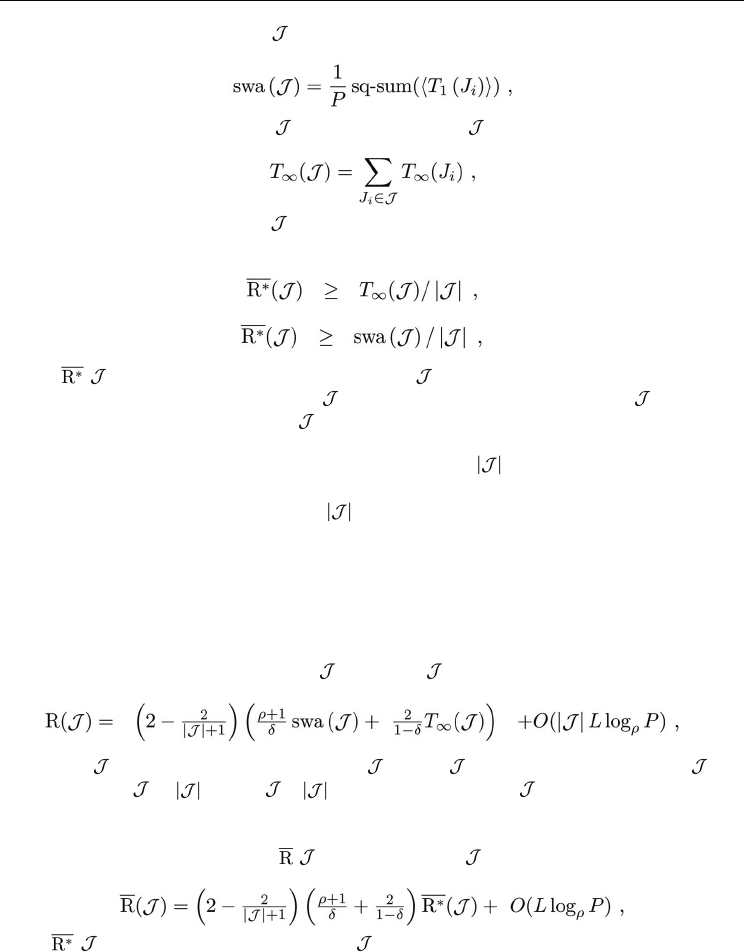
The squashed work area of a job set
on a set of P processors is
where T
1
(J
i
) is the work of job J
i
∈ . The aggregate span of is
where T
∞
(J
i
) is the span of job J
i
∈ .
The research in [36, 37, 10] establishes two lower bounds for the mean response time:
(4)
(5)
where
( ) denotes the mean response time of scheduled by an optimal clairvoyant
scheduler. Both the aggregate span T
∞
( ) and the squashed work area swa ( ) are lower
bounds of the total response time R*(
) under an optimal clairvoyant scheduler.
Analysis
The proof is divided into two parts. In the first part where ≤ P, GRAD always uses DEQ
as job scheduler. In this case, we apply the result in [18], and show that GRAD is O(1)-
competitive. In the second part where > P, GRAD uses both RR and DEQ. Since we
consider batched jobs, the number of incomplete jobs decreases monotonically. When the
number of incomplete jobs drops to P, GRAD switches its job scheduler from RR to DEQ.
Therefore, we prove the second case based on the properties of round robin scheduling and
the results of the first case. The following theorem shows the total response time bound for
the batched job sets scheduled by GRAD. Please refer to Appendix A for the complete proof.
Theorem 4 Let ρ be A-GREEDY's responsiveness parameter, its utilization parameter, and L the
quantum length. The total response time R(
) of a job set produced by GRAD is at most
(6)
where swa (
) denotes the squashed work area of , and T
∞
( ) denotes the aggregate span of . □
Since both swa ( ) / and T
∞
( )/ are lower bounds on R( ), we obtain the following
corollary. It shows that GRAD is O(1)-competitive with respect to mean response time for
batched jobs.
Corollary 5 The mean response time ( ) of a batched job set produced by GRAD satisfies
where ( ) denotes the mean response time of scheduled by an optimal clairvoyant scheduler. □
6. Experimental results
To evaluate the performance of GRAD, we conducted four sets of experiments, which are
summarized below.
Advances in Greedy Algorithms
446
• The makespan experiments compares the makespan produced by GRAD against the
theoretical lower bound for over 10000 runs of job sets.
• The mean response time experiments investigate how GRAD performs with respect to
mean response time for over 8000 batched job sets.
• The load experiments investigate how the system load affects the performance of
GRAD.
• The proactive RAD experiments compare the performance of RAD against its variation
- proactive RAD. The proactive RAD always allots all processors to jobs even if the
overall desire is less than the total number of processors.
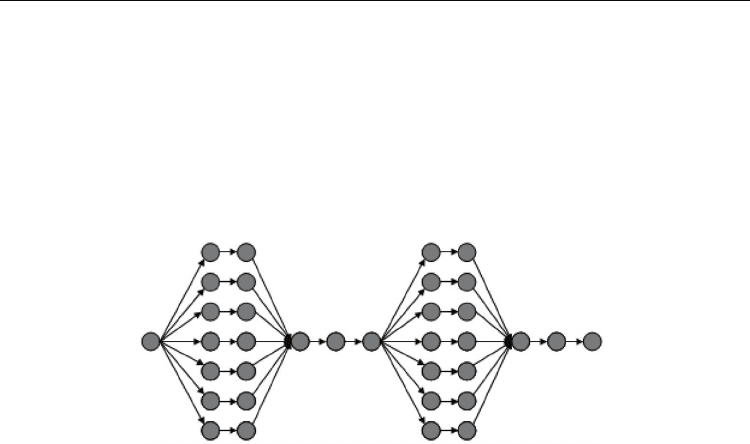
Fig. 1. The DAG of a fork-join job used in the simulation. This job has start-up length w
0
= 1,
serial phase length w
1
= 3, parallel phase length w
2
= 2, parallelism h = 7, and the number of
iterations iter = 2.
6.1 Simulation setup
To study GRAD, we build a Java-based discrete-time simulator using DESMO-J [11]. Our
simulator models four major entities - processors, jobs, thread schedulers, and job
schedulers, and simulates their interactions in a two-level scheduling environment. As
described in Section 2, we model the execution of a multithreaded job as a dag. When a job
is submitted to the simulated multiprocessor system, an instance of a thread scheduler is
created for the job. The job scheduler allots processors to the job, and the thread scheduler
executes the job using A-GREEDY. The simulator operates in discrete time steps, and we
ignore the overheads incurred in the reallocation of processors.
Our benchmark application is the Fork-Join jobs, whose task graphs are typically as shown
in Figure 1. Each job alternates between a serial phase of length w
1
and a parallel phase (with h-
way parallelism) of length w
2
, while the initial serial phase has length w
0
. The parallelism of
job's parallel phase is the height h of the job, and the number of iterations is denoted as iter .
Fork-Join jobs arise naturally in jobs that exhibit “data parallelism”, and apply the same
computation to a number of different data points. Many computationally intensive
applications can be expressed in a data-parallel fashion [30]. The repeated fork-join cycle in
the job reflects the often iterative nature of these computations. The average parallelism of
the job is approximately (w
1
+ hw
2
)=(w
1
+ w
2
). By varying the values of w
0
, w
1
, w
2
, h, and the
number of iterations, we can generate jobs with different work, spans, and phase lengths.
GRAD requires some parameters as input. We set the responsiveness parameter to be ρ= 2.0,
and the utilization parameter = 0.8 unless otherwise specified. GRAD is designed for
moderate-scale and large-scale multiprocessors, and we set the number of processors to be
P = 128. The quantum length L represents the time between successive reallocations of
Provably-Efficient Online Adaptive Scheduling of Parallel Jobs Based on Simple Greedy Rules
447
processors by the job scheduler, and is selected to amortize the overheads due to the
communication between the job scheduler and the thread scheduler, and the reallocation of
processors. In conventional computer systems, a scheduling quantum is typically between
10 and 20 milliseconds. The execution time of a task is decided by the granularity of the job.
If a task takes approximately 0.5 to 5 microseconds, then the quantum length L should be set
to values between 10
3
and 10
5
time steps. Our theoretical bounds indicate that as long as
T
∞
Llog P, the length of L should have little effect on our results. In our experiments, we
set L = 1000.
6.2 Makespan experiments
The competitive ratio of makespan derived in Section 4, though asymptotically strong, has a
relatively large constant multiplier. The makespan experiments were designed to evaluate
the constants that would occur in practice and compare GRAD to an optimal scheduler. The
experiments are conducted on more than 10, 000 runs of job sets using many combinations
of jobs and different loads.
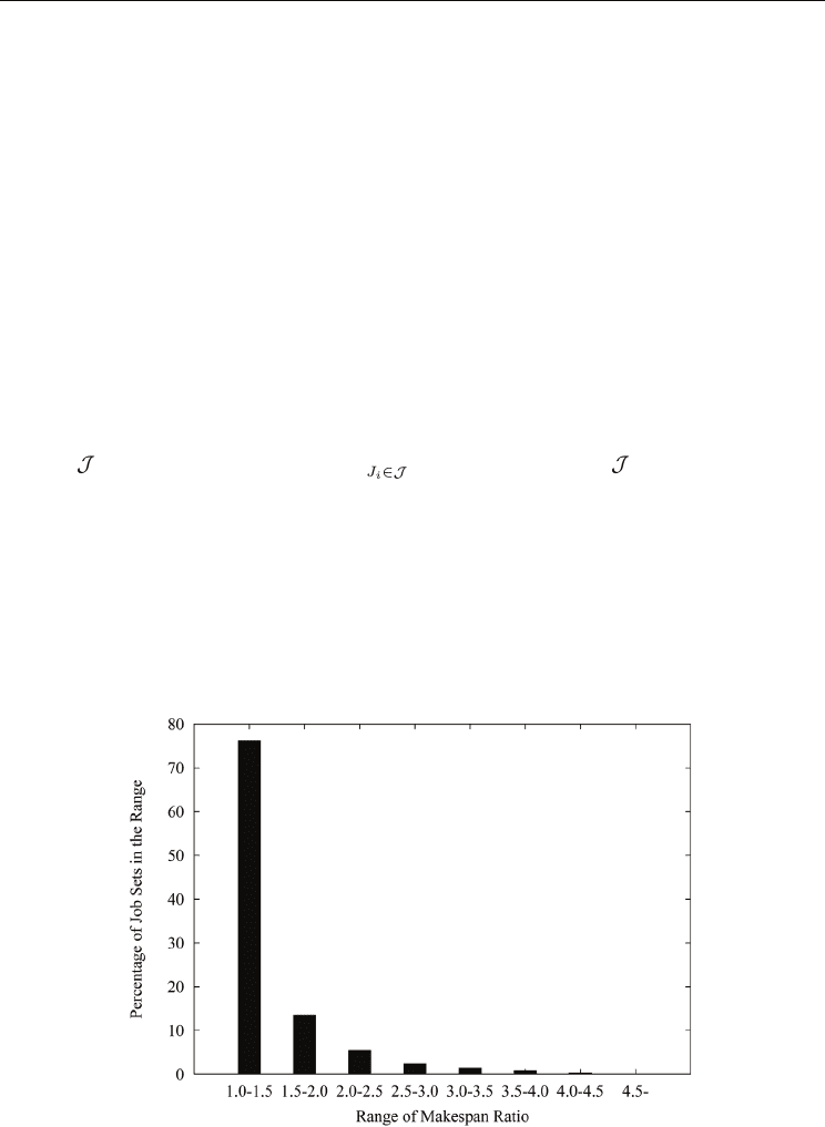
Figure 2 shows how GRAD performs compared to an optimal scheduler. The makespan of a
job set
has two lower bounds max (r(J
i
) + T
∞
(J
i
)) and T
1
( ) =P. The makespan
produced by an optimal scheduler is lower-bounded by the larger of these two values. The
makespan ratio in Figure 2 is defined as the makespan of a job set scheduled by GRAD
divided by the theoretical lower bounds. Its X-axis represents the range of the makespan
ratio, while the histogram shows the percentage of the job sets whose makespan ratio falls
into the range. Among more than 10, 000 runs, 76.19% of them use less than 1.5 times of the
theoretical lower bound, 89.70% use less than 2.0 times, and none uses more than 4.5 times.
The average makepsan ratio is 1.39, which suggests that, in practice, GRAD has a small
competitive ratio with respect to the makespan.
Fig. 2. Comparing the makespan of GRAD with the theoretical lower bound for job sets with
arbitrary job release time.
Advances in Greedy Algorithms
448
We now interpret the relation between the theoretical bounds and experimental results as
follows. When ρ = 2 and = 0.8, from Theorem 2, GRAD is 13.75-competitive in the worst
case. However, we anticipate that GRAD's makespan ratio would be small in practical
settings, especially when the jobs have total work much great than the span and with the
machine moderately- or highly- loaded. In this case, the term on T
1
( )/P in Inequality (3) of
Theorem 2 is much larger than the term max
{T
∞
(i) + r(i)}, i.e. the term T
1
( )/P
generally dominates the makespan bound. The proof of Theorem 2 calculates the coefficient
of T
1
( )/P as the ratio of the total allotment (total work plus total waste) versus the total
work. When the job scheduler is RAD, which is not a true adversary, our simulation results
indicate that the ratio of the waste versus the total work is only about 1/10 of the total work.
Thus, the coefficient of T
1
( )/P in Inequality (3) is about 1.1. It explains why the makespan
produced by GRAD is less than 2 times of the lower bound on average as shown in Figure 2.
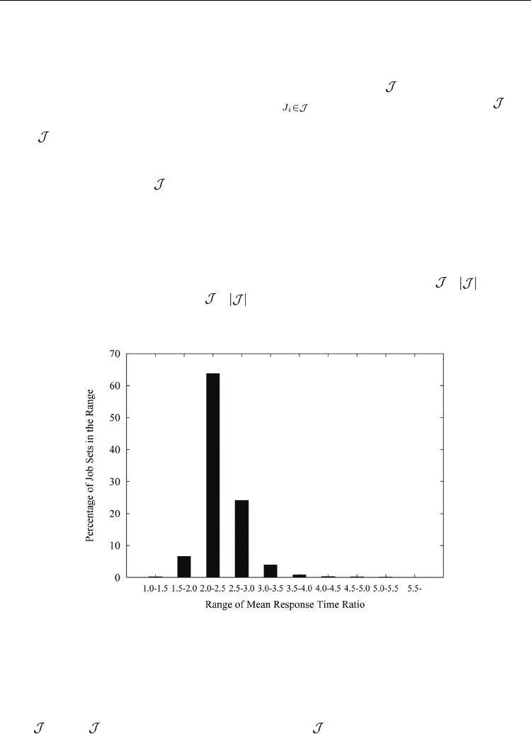
6.3 Mean response time experiments
This set of experiments is designed to evaluate the mean response time of the batch job sets
scheduled by GRAD. Figure 3 shows the distribution of the mean response time normalized
w.r.t. the larger of the two lower bounds { the squashed work bound swa (
) / and the
aggregated critical path bound T
∞
( )/ . The histogram in Figure 3 shows that, among
more than 8, 000 runs, 94.65% of them use less than 3 times of the theoretical lower bound,
and none of them uses more than 5:5 times. The average mean response time ratio is 2.37.
Fig. 3. Comparing the mean response time of GRAD with the theoretical lower bound for
batched job sets.
Similar to the discussion in Section 6.2, we can relate the theoretical bounds for mean
response time to the experimental results. When ρ = 2 and ρ = 0.8, from Theorem 4, GRAD is
27.60-competitive. However, we expect that GRAD should perform closer to optimal in
practice. In particular, when the job set J exhibits reasonably large total parallelism, we have
swa (
) T
∞
( ), and thus, the term involving swa ( ) in Theorem 4 dominates the total
response time. More importantly, RAD is not an adversary of A-GREEDY, as mentioned
Provably-Efficient Online Adaptive Scheduling of Parallel Jobs Based on Simple Greedy Rules
449
before, the waste of a job is only about 1/10 of the total work in average for over 100, 000 job
runs we tested. Based on this waste, the squashed area bound swa (
) in Inequality (6) of
Theorem 4 has a coefficient to be around 2.2. It explains that the mean response time
produced by GRAD is less than 3 times of the lower bound as shown in Figure 3.
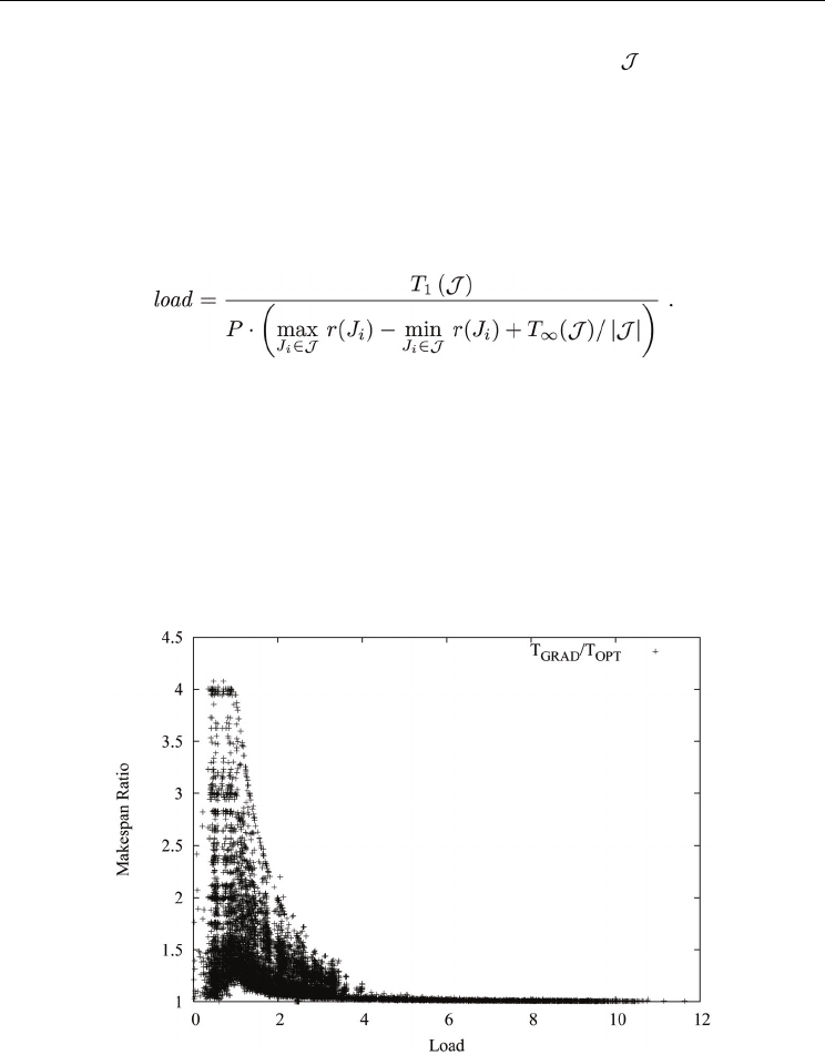
6.4 Load experiments
This set of experiments is designed to investigate how the load affects the performance of
GRAD. The load of a job set J on a machine with P processors indicates how heavily the jobs
compete for processors on the machine, which is calculated as follows
For a batched job set, the load is just the average parallelism of the set divided by the total
number of processors.
Figure 4 shows how GRAD performs against the theoretical lower bound with respect to
makespan by varying system load. The makespan ratio in this figure is defined as the
makespan of a job set scheduled by GRAD divided by the larger of the two lower bounds.
Each data point represents the makespan ratio of a job set. The testing results suggest that
the makespan ratio becomes smaller when the load gets heavier. Specifically, the makespan
generated by GRAD is very close to the lower bound when the load is greater than 4; it
never exceeds 1.5 times of the makespan produced when the system load is greater than 3.
However, when the load is less than 2, the makespan ratio spreads in the range from 1 to 4.
Fig. 4. Comparing GRAD against the theoretical lower bound for makespan with varying
load.
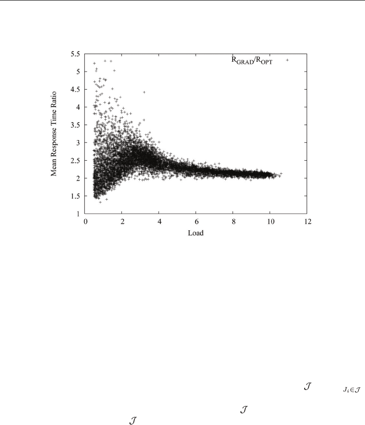
Figure 5 shows the performance of GRAD with respect to mean response time for batched
jobs by varying system load. It compares the mean response time incurred by GRAD with
Advances in Greedy Algorithms
450
the theoretical lower bound. Under heavy load, the mean response time produced by GRAD
concentrates on about 2 times of the lower bound, while under light load, the ratio spreads
in the range from 1 to 4.
Fig. 5. Comparing GRAD against the theoretical lower bound for mean response time with
varying load for batched jobs.
The load experiments bring up a question of how to improve the performance of GRAD
under light load. The job scheduler RAD makes conservative decision on the allocation of
processors to jobs. When the system is lightly loaded where the total demand is less than the
total number of processors, RAD keeps some processors idle without allocating them to any
jobs. Since a greedy thread scheduler executes a job faster with more processors allotted, a
job scheduler that always allots all processors to jobs should perform better under light load.
We will explore such a variation of the job scheduler RAD in the next set of the experiments.
6.5 Proactive RAD experiments
Proactive RAD always allocates all processors to jobs even if the total requests are less than
the total number of processors. At a quantum q, when the total requests d( , q) = Σ
d(J
i
, q) are greater than or equal to the total number P of processors, the proactive RAD
works exactly the same as the original one. However, if d( , q) < P, the proactive RAD
evenly allots the remaining P - d( , q) processors to all the jobs.
Figure 6 shows the makespan ratio of proactive RAD against its original algorithm by
varying system load. Each data point in the figure represents a job set's makespan ratio,
defined as the makespan produced by the proactive RAD divided by that of the original. We
can see that the makespan ratio is less than 1 for most of the runs, indicating that the
proactive RAD out-performs the original one in most of these job sets. Moreover, the
difference between them becomes more pronounced under light load, and diminishes with
the increase of the system load. The reason is that the proactive RAD generally allocates
more processors to jobs, especially when the load is light. The increased allotment allows