Baumgarte T., Shapiro S. Numerical Relativity. Solving Einstein’s Equations on the Computer

Подождите немного. Документ загружается.

2.3 Foliations of spacetime 31

Thus γ

is a projection tensor that projects out all geometric objects lying along n

This metric allows us to compute distances within a slice . To see that γ

is purely

spatial, i.e., resides entirely in  with no piece along n

, we contract it with the

normal n

= n

+ n

= n

− n

= 0. (2.28)

Intuitively, γ

calculates the spacetime distance with g

and then kills off the timelike

contribution (normal to the spatial surface) with n

. The inverse spatial metric can be

found by raising the indices of γ

with g

= g

+ n

. (2.29)

Next we break up 4-dimensional tensors by decomposing them into a purely spatial

part, which lies in the hypersurfaces , and a timelike part, which is normal to the spatial

surface. To do so, we need two projection operators. The ﬁrst one, which projects a 4-

dimensional tensor into a spatial slice, can be found by raising only one index of the spatial

metric γ

= g

+ n

= δ

+ n

. (2.30)

Exercise 2.6 Show that γ

,wherev

is an arbitrary spacetime vector, is purely

spatial.

To project higher rank tensors into the spatial surface, each free index has to be contracted

with a projection operator. It is sometimes convenient to denote this projection with a

symbol ⊥, e.g.,

⊥ T

= γ

. (2.31)

Similarly, we may deﬁne the normal projection operator as

≡−n

= δ

− γ

, (2.32)

even though in most cases it is just as easy to write out the normal vectors n

.We

can now use these two projection operators to decompose any tensor into its spatial and

timelike parts. For example, we can write an arbitrary vector v

= δ

= (γ

+ N

=⊥ v

− n

. (2.33)

Exercise 2.7 Show that for the second rank tensor T

we have

=⊥ T

− n

⊥ T

− n

⊥ T

+ n

. (2.34)

Exercise 2.7 illustrates that the ⊥ symbol has to be used with some care, since it applies

only to the free indices of the tensor that it operates on. To avoid confusion, we will usually

write out the projection operators explicitly.

32 Chapter 2 The 3+1 decompostion of Einstein’s equations

It may be useful to illustrate the above concepts for a familiar example. Consider a

Schwarzschild spacetime in isotropic spherical polar coordinates

=−



1 − M/(2r)

1 + M/(2r)





1 +



(dr

dθ

sin

θdφ

) (2.35)

and identify the spatial slices  with hypersurfaces of constant coordinate time t. Then

the components of the 1-form 

in a coordinate basis are simply



= (1, 0, 0, 0) (2.36)

and from its normalization (2.21)weﬁndthelapse

α =

1 − M/(2r)

1 + M/(2r)

. (2.37)

The normal vector n

is then

=−g

1 + M/(2r)

1 − M/(2r)

(1, 0, 0, 0), (2.38)

and the spatial metric (2.27) becomes



1 +



diag



0, 1, r

, r

sin



. (2.39)

It is evident that this metric eliminates any t-components.

Returning to our formal derivation of the 3 + 1 decomposition we will also need a

3-dimensional covariant derivative that maps spatial tensors into spatial tensors. It is

uniquely deﬁned by requiring that it be compatible with the 3-dimensional metric γ

.We

can construct this derivative by projecting all indices present in a 4-dimensional covariant

derivative into . For a scalar f , for example, we deﬁne

f ≡ γ

∇

f, (2.40)

and for a rank (

)tensorT

≡ γ

∇

. (2.41)

The extension to other type tensors is obvious.

Exercise 2.8 Show that the 3-dimensional covariant derivative is compatible with

the spatial metric γ

, that is, show that

= 0. (2.42)

Exercise 2.9 Show that for a scalar product v

, the Leibnitz rule

) = v

+ w

(2.43)

holds only if v

and w

are purely spatial.

See, e.g., Misner et al. (1973), equation (31.22).

2.4 The extrinsic curvature 33

δn

∝−K

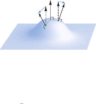
Figure 2.2 The extrinsic curvature of a hypersurface in an enveloping spacetime measures how much normal

vectors to the hypersurface differ at neighboring points. It therefore measures the rate at which the hypersurface

warps as it is carried forward along a normal vector.

The 3-dimensional covariant derivative can be expressed in terms of 3-dimensional

connection coefﬁcients, which, in a coordinate basis, are given by



(∂

+ ∂

− ∂

). (2.44)

The 3-dimensional Riemann tensor associated with γ

is deﬁned by requiring that

= R

cba

= 0 (2.45)

for any spatial vector w

. In a coordinate basis, the components of the Riemann tensor can

be computed from

abc

= ∂



− ∂



+ 



− 



. (2.46)

Contracting the Riemann tensor yields the 3-dimensional Ricci tensor R

= R

acb

and the

3-dimensional Ricci scalar R = R

Einstein’s equations (1.32) relate contractions of the 4-dimensional Riemann tensor

(4)

bcd

to the stress–energy tensor. Since we want to rewrite these equations in terms of

3-dimensional objects, we decompose

(4)

bcd

into spatial tensors. Not surprisingly, this

decomposition involves its 3-dimensional cousin R

bcd

, but obviously this cannot contain

all the information needed. R

abc

is a purely spatial object and can be computed from spatial

derivatives of the spatial metric alone, while

(4)

abc

is a spacetime creature which also

contains time derivatives of the 4-dimensional metric. Stated differently, the 3-dimensional

curvature R

bcd

only contains information about the curvature intrinsic to a slice ,butit

gives no information about what shape this slice takes in the spacetime M in which it is

embedded. This information is contained in a tensor called the extrinsic curvature.

2.4 The extrinsic curvature

The extrinsic curvature K

can be found by projecting gradients of the normal vector

into the slice  (see Figure 2.2). We will also see that the extrinsic curvature is related to

See equation (1.20) for the 4-dimensional analog of this expression.

34 Chapter 2 The 3+1 decompostion of Einstein’s equations

the ﬁrst time derivative of the spatial metric γ

. The metric and the extrinsic curvature

(γ

, K

) can therefore be considered as the equivalent of positions and velocities in

classical mechanics – they measure the “instantaneous” state of the gravitational ﬁeld,

and form the fundamental variables in our initial value formulation. Mathematicians often

refer to the metric as the ﬁrst, and the extrinsic curvature the second, fundamental form.

The projection of the gradient of the normal vector γ

∇

can be split into a

symmetric part, also known as the expansion tensor

= γ

∇

, (2.47)

and an antisymmetric part, also known as the rotation 2-form or twist,

= γ

∇

. (2.48)

Exercise 2.10 Show that the twist ω

has to vanish as a consequence of n

being

rotation-free (see exercise 2.5).

We now deﬁne the extrinsic curvature, K

, as the negative expansion

≡−γ

∇

=−γ

∇

. (2.49)

By deﬁnition, the extrinsic curvature is symmetric and purely spatial. It measures the

gradient of the normal vectors n

. Since the latter are normalized, they can only differ

in the direction in which they are pointing, and the extrinsic curvature therefore provides

information on how much this direction changes from point to point across a spatial hyper-

surface, as illustrated in Figure 2.2. As a consequence, the extrinsic curvature measures

the rate at which the hypersurface deforms as it is carried forward along a normal.

Exercise 2.11 Show that the extrinsic curvature of t = constant hypersurfaces of

the Schwarzschild metric (2.35)vanishes.

Alternatively, we can express the extrinsic curvature in terms of the acceleration of the

unit normal vector ﬁeld

≡ n

∇

. (2.50)

Exercise 2.12 Show that the acceleration a

is purely spatial, n

= 0.

Exercise 2.13 Show that the acceleration a

is related to the lapse α according to

= D

ln α. (2.51)

Exercise 2.14 Find the acceleration a

for the normal observer (2.38) in a Schwarz-

schild spacetime.

Expanding the right hand side of (2.49) and using the identity n

∇

= 0 together with

the deﬁnition of a

we ﬁnd

=−γ

∇

=−(δ

+ n

)(δ

+ n

)∇

=−(δ

+ n

)δ

∇

=−∇

− n

. (2.52)

2.4 The extrinsic curvature 35

Finally, we can write the extrinsic curvature as

=−

, (2.53)

where

denotes the Lie derivative along n

. The concept and properties of the Lie

derivative are sketched in Apppendix A. Here we simply note that the Lie derivative along

a vector ﬁeld X

measures by how much the changes in a tensor ﬁeld along X

differ from

a mere inﬁnitesimal coordinate transformation generated by X

. For a scalar f , the Lie

derivative reduces to the partial derivative

f = X

∂

f ; (2.54)

for a vector ﬁeld v

the Lie derivative is the commutator, so that in a coordinate basis,

= X

∂

− v

∂

= [X,v]

, (2.55)

and for a 1-form ω

the Lie derivative is given by

= X

∂

+ ω

∂

. (2.56)

It then follows that for a tensor T

of rank (

) the Lie derivative is

= X

∂

− T

∂

+ T

∂

. (2.57)

Generalization to tensors of arbitrary rank follows naturally. Lie differentiation satisﬁes

the chain rule and the usual addition properties obeyed by covariant differentiation. Also,

in all of the above expressions for the Lie derivative one may replace the partial derivatives

with covariant derivatives.

Since n

is a timelike vector, equation (2.53) illustrates the intuitive interpretation of

the extrinsic curvature as a geometric generalization of the “time derivative” of the spatial

metric γ

. Obviously, the spatial metric γ

on two different slices  may differ by virtue of

a coordinate transformation. Equation (2.53) states that, in addition to a mere coordinate

transformation (which by itself would yield

= 0, see Appendix A), γ

changes

proportionally to K

To derive equation (2.53), we write γ

in terms of g

and n

and use (A.13) and (A.19):

= L

+ n

) = 2∇

+ n

= 2(∇

+ n

) =−2K

. (2.58)

The last equality results from equation (2.52). The extrinsic curvature is often deﬁned

by equation (2.53), from which our deﬁnition (2.49)aswellas(2.52) can be derived.

Obviously, this logical development is completely equivalent and the choice is merely a

matter of taste.

The trace of the extrinsic curvature, often called the mean curvature,

K = g

= γ

, (2.59)

36 Chapter 2 The 3+1 decompostion of Einstein’s equations

also has a nice geometrical interpretation. To see this, we take the trace of (2.53)toﬁnd

K = γ

=−

2γ

γ =−

1/2

=−L

ln γ

1/2

. (2.60)

Since γ

1/2

x is the proper volume element in the spatial slice , the negative of the mean

curvature measures the fractional change in the proper 3-volume along n

2.5 The equations of Gauss, Codazzi and Ricci

The metric γ

and the extrinsic curvature K

cannot be chosen arbitrarily. Instead, they

have to satisfy certain constraints, so that the spatial slices “ﬁt” into the spacetime M.In

order to ﬁnd these relations, we have to relate the 3-dimensional Riemann tensor R

bcd

of the hypersurfaces  to the 4-dimensional Riemann tensor

(4)

bcd

of M.Todoso,

we ﬁrst take a completely spatial projection of

(4)

bcd

, then a projection with one index

projected in the normal direction, and ﬁnally a projection with two indices projected in

the normal direction. All other projections vanish identically because of the symmetries of

the Riemann tensor. A decomposition of

(4)

bcd

into spatial and normal pieces therefore

involves these three different types of projections.

Exercise 2.15 Following the example of exercise 2.7, show that the 4-dimensional

Riemann tensor

(4)

abcd

can be written as

(4)

abcd

= γ

(4)

pqrs

− 2γ

s (4)

pqrs

−2γ

s (4)

pqrs

+ 2γ

s (4)

pqrs

−2γ

s (4)

pqrs

. (2.61)

The above projections give rise to the equations of Gauss, Codazzi and Ricci, which we

will derive below. Given that

(4)

bcd

involves up to second time derivatives of the metric,

while R

bcd

only contains space derivatives, we may already anticipate that these relations

will involve the extrinsic curvature and its time derivative.

The Riemann tensor is deﬁned in terms of second covariant derivatives of a vector. To

relate the 4-dimensional Riemann tensor to its 3-dimensional counterpart, it is therefore

natural to start by relating the corresponding covariant derivatives to each other. We ﬁrst

expand the deﬁnition of the spatial gradient of a spatial vector V

= γ

∇

= γ

+ n

)∇

= γ

∇

− γ

∇

= γ

∇

− n

∇

= γ

∇

+ n

, (2.62)

wherewehaveusedn

= 0, and hence n

∇

=−V

∇

, as well the deﬁnition of

the extrinsic curvature (2.49).

See also Poisson (2004), Section 2.3.8. Alternatively, from equation (2.49)or(4.7)wehavethatK =−∇

−(1/V )dV/dτ , hence K measures the expansion of normal observers, or the fractional rate of change, with respect to

proper time τ , of the proper volume V of a bundle of normal observers; see, e.g., Misner et al. (1973), equation (22.2).

2.5 The equations of Gauss, Codazzi and Ricci 37

Exercise 2.16 Show that

∇

(αV

) (2.63)

for any spatial vector V

Hint: One possible derivation uses equations (2.51)and(2.62); a more elegant

approach starts with the identity (A.44).

Exercise 2.17 Show that

= γ

∇

− K

∇

− K

. (2.64)

We can now use equation (2.64) to relate the 3- and 4-dimensional Riemann tensors to

each other. Writing the deﬁnition of the 3-dimensional Riemann tensor (2.45)as

= 2D

(2.65)

we can insert the second derivative (2.64)toﬁnd

= 2γ

∇

− 2K

[ab]

∇

− 2K

b] p

. (2.66)

The second term on the right hand side vanishes because K

is symmetric, and the ﬁrst

term can be rewritten in terms of the 4-dimensional Riemann tensor, which yields

dcba

= γ

(4)

drqp

− 2K

c[a

b]d

(2.67)

after relabeling some indices and lowering the index c. Since this relation has to hold for

any arbitrary spatial vector V

,wehave

abcd

+ K

− K

= γ

(4)

pqrs

. (2.68)

This equation is called Gauss’ equation. It relates the full spatial projection of

(4)

bcd

the 3-dimensional R

bcd

and terms quadradic in the extrinsic curvature.

Next, we want to consider projections of

(4)

bcd

with one index projected in the normal

direction. This will involve a spatial derivative of the extrinsic curvature

= γ

∇

=−γ

(∇

∇

+∇

)). (2.69)

Since γ

= 0, only the gradient of n

will give a nonzero contribution in the second

term, namely

∇

=−a

. (2.70)

We therefore have

=−γ

∇

+ a

. (2.71)

Since K

is symmetric, the last term disappears when antisymmetrizing to give

b]c

=−γ

∇

. (2.72)

38 Chapter 2 The 3+1 decompostion of Einstein’s equations

By the deﬁnition of the Riemann tensor, this can be rewritten as

− D

= γ

s (4)

pqrs

. (2.73)

This equation is known as the Codazzi equation. Note that Gauss’ equation (2.68)and

the Codazzi equation (2.73) depend only on the spatial metric, the extrinsic curvature

and their spatial derivatives. They can be thought of as the integrability conditions allow-

ing the embedding of a 3-dimensional slice  with data (γ

, K

) inside a 4-dimensional

manifold M with g

. As we will see in the next section, these two equations give rise to

the “constraint” equations.

However, before deriving the constraint equations in the next section, we ﬁrst consider

the last remaining projection of

(4)

bcd

, namely with two indices projected in the normal

direction. This will involve a “time” derivative of K

, and therefore we ﬁrst compute

= n

∇

+ 2K

c(a

∇

=−n

∇

− n

∇

) − 2K

c(a

− 2K

c(a

. (2.74)

Here we have used equation (2.52) to expand both terms. We can now insert

(4)

dbac

= 2∇

∇

, (2.75)

which yields

=−n

c (4)

dbac

− n

∇

− n

∇

−

∇

− 2K

b)c

− 2K

c(a

. (2.76)

Using the deﬁnition of a

= n

∇

and the relation

∇

=∇

− (∇

)(∇

) =∇

− K

− n

(2.77)

several terms cancel and we ﬁnd

=−n

c (4)

dbac

−∇

− n

∇

− a

− K

. (2.78)

Exercise 2.18 Show that L

is purely spatial,

= 0. (2.79)

Since L

is purely spatial, projecting the two free indices in (2.78)leavestheleft

hand side unchanged and results in

=−n

(4)

drqc

− γ

∇

− a

− K

. (2.80)

Exercise 2.19 Show that

=−a

α. (2.81)

2.6 The constraint and evolution equations 39

Finally, we simplify (2.80) with the help of equation (2.81), and ﬁnd

= n

(4)

drcq

−

α − K

. (2.82)

Equation (2.82) is Ricci’s equation.

It relates the “time” derivative of K

to a pro-

jection of the 4-dimensional Rieman tensor with two indices projected in the “time”

direction.

2.6 The constraint and evolution equations

Now we have assembled all the necessary tools, and can rewrite Einstein’s ﬁeld

equations in a 3 + 1 form. Basically, we just need to take the equations of Gauss,

Codazzi and Ricci and eliminate the 4-dimensional Rieman tensor using Einstein’s

equations

≡

(4)

−

(4)

= 8π T

. (2.83)

The last few sections dealt with purely geometrical objects; we will now invoke Ein-

stein’s equations to link these geometrical objects to physical properties of spacetimes.

We will ﬁrst derive the constraint equations from Gauss’ equation (2.68) and the Codazzi

equation (2.73), and will then derive the evolution equations from (2.53) and the Ricci

equation (2.82).

Contracting Gauss’ equation (2.68) once, we ﬁnd

(4)

pqrs

= R

+ KK

− K

, (2.84)

where K is the trace of the extrinsic curvature, K = K

. A further contraction yields

qs (4)

pqrs

= R + K

− K

. (2.85)

The left hand side can be expanded into

qs (4)

pqrs

= (g

+ n

)(g

+ n

)

(4)

pqrs

(4)

R + 2n

r (4)

. (2.86)

Note that the term n

s (4)

pqrs

vanishes identically because of the symmetry prop-

erties of the Riemann tensor. We also have

= 2n

r (4)

− n

(4)

R = 2n

r (4)

− n

(γ

− n

)

(4)

= 2n

r (4)

(4)

R = γ

qs (4)

pqrs

, (2.87)

In the general relativity literature, equations (2.68)and(2.73) are often jointly referred to as the Gauss–Codazzi

equations. In the differential geometry literature, however, (2.68) is known as the Gauss equation (which represents a

generalization of Gauss’s Theorema Egregium), while (2.73) is called the Codazzi or Codazzi–Mainardi relation.The

name Ricci equation for (2.82) is also more commonly used in differential geometry books than in general relativity

books.

40 Chapter 2 The 3+1 decompostion of Einstein’s equations

wherewehaveusedequation(2.86) in the last equality. Inserting this into the contracted

Gauss’ equation (2.85) yields

= R + K

− K

. (2.88)

We now deﬁne the energy density ρ to be the total energy density as measured by a normal

observer n

ρ ≡ n

. (2.89)

Using Einstein’s equation (2.83) together with equations (2.88) and (2.89), we obtain

R + K

− K

= 16πρ. (2.90)

Equation (2.90)istheHamiltonian constraint.

Contracting the Codazzi equation (2.73) once yields

− D

K = γ

s (4)

pqrs

. (2.91)

The right hand side is

s (4)

pqrs

=−γ

+ n

s (4)

qprs

=−γ

s (4)

− γ

s (4)

qprs

(2.92)

The last term vanishes again because of the symmetries of

(4)

efgd

, while the ﬁrst term on

the right hand side can be rewritten using

= γ

s (4)

−

(4)

R = γ

s (4)

. (2.93)

Here the last equality holds because γ

= γ

= 0. Collecting terms and inserting

into equation (2.91) we obtain

− D

K =−γ

. (2.94)

We now deﬁne S

to be the momentum density as measured by a normal observer n

≡−γ

, (2.95)

and ﬁnd

− D

K = 8π S

. (2.96)

Equation (2.96)isthemomentum constraint.

Exercise 2.20 Consider a swarm of particles of rest-mass m and proper (comoving)

number density n, all moving with the same 4-velocity u

. The stress-energy tensor

for such a swarm is T

= mnu

. Determine the energy density ρ and momentum

density S

for the swarm and provide a simple physical interpretation for the terms

in your expressions.