Articolo G.A. Partial Differential Equations and Boundary Value Problems with Maple V
Подождите немного. Документ загружается.


388 Chapter 6
> mu[m]:=m*Pi/b;
μ
m
:= m (6.111)
for m = 1, 2, 3,....
Eigenvalues λ
m,n
are the roots of the eigenvalue equation
> BesselJ(mu[m],lambda[m,n]*a)=0;
BesselJ(m, λ
m,n
) = 0 (6.112)
for m = 1, 2, 3,..., n= 1, 2, 3,....
Orthonormal eigenfunctions
> R[m,n](r):=BesselJ(mu[m],lambda[m,n]*r)/sqrt(Int(BesselJ(mu[m],lambda[m,n]*r)ˆ2*r,
r=0..a));R[m,p](r):=subs(n=p,R[m,n](r)):
R
m,n
(r) :=
BesselJ(m, λ
m,n
r)
1
0
BesselJ(m, λ
m,n
r)
2
r dr
(6.113)
> phi[m](theta):=sqrt(1/Pi)*cos(m*theta);phi[q](theta):=subs(m=q,phi[m](theta)):
φ
m
(θ) :=
cos(mθ)
√
π
(6.114)
> psi[m](theta):=sqrt(1/Pi)*sin(m*theta);psi[q](theta):=subs(m=q,psi[m](theta)):
m
(θ) :=
sin(mθ)
√
π
(6.115)
For m = 0, the eigenvalues are the roots of the equation
> BesselJ(0,lambda[0,n]*a)=0;
BesselJ(0,λ
0,n
) = 0 (6.116)
Orthonormal eigenfunctions
> R[0,n](r):=BesselJ(0,lambda[0,n]*r)/sqrt(Int(BesselJ(0,lambda[0,n]*r)ˆ2*r,r=0..a));
R[0,p](r):=subs(n=p,R[0,n](r)):
R
0,n
(r) :=
BesselJ(0,λ
0,n
r)
1
0
BesselJ(0,λ
0,n
r)
2
r dr
(6.117)
> phi[0](theta):=1/sqrt(2*Pi);
φ
0
(θ) :=
1
2
√
2
√
π
(6.118)

The Diffusion Equation in Two Spatial Dimensions 389
Statements of orthonormality with their respective weight functions
> w(r):=r:Int(R[m,n](r)*R[m,p](r)*w(r),r=0..a)=delta(n,p);
1
0
BesselJ(m, λ
m,n
r)BesselJ(m, λ
m,p
r)r
1
0
BesselJ(m, λ
m,n
r)
2
r dr
1
0
BesselJ(m, λ
m,p
r)
2
r dr
dr = δ(n, p) (6.119)
> w(theta):=1:Int(phi[m](theta)*phi[q](theta)*w(theta),theta=−Pi..Pi)=delta(m,q);
π
−π
cos(mθ) cos(qθ)
π
dθ = δ(m, q) (6.120)
> w(theta):=1:Int(psi[m](theta)*psi[q](theta)*w(theta),theta=−Pi..Pi)=delta(m,q);
π
−π
sin(mθ) sin(qθ)
π
dθ = δ(m, q) (6.121)
Time-dependent solution
> T[m,n](t):=exp(−k*lambda[m,n]ˆ2*t);u[m,n](r,theta,t):=T[m,n](t)*R[m,n](r)*(A(m,n)
*phi[m](theta)+B(m,n)*psi[m](theta)):
T
m,n
(t) := e
−
1
50
λ
2
m,n
t
(6.122)
> T[0,n](t):=A(0,n)*exp(−k*lambda[0,n]ˆ2*t);u[0,n](r,theta,t):=T[0,n](t)*R[0,n](r)
*phi[0](theta):
T
0,n
(t) := A(0,n)e
−
1
50
λ
2
0,n
t
(6.123)
Eigenfunction expansion
> u(r,theta,t):=Sum(u[0,n](r,theta,t),n=1..infinity)+Sum(Sum(u[m,n](r,theta,t),m=1..infinity),
n=1..infinity);
u(r,θ,t):=
∞
n=1
1
2
A(0,n)e
−
1
50
λ
2
0,n
t
BesselJ(0,λ
0,n
r)
√
2
1
0
BesselJ(0,λ
0,n
r)
2
rdr
√
π
+
∞
n=1
⎛
⎜
⎝
∞
m=1
e
−
1
50
λ
2
m,n
t
BesselJ(m, λ
m,n
r)
A(m,n) cos(mθ)
√
π
+
B(m,n) sin(mθ)
√
π
1
0
BesselJ(m, λ
m,n
r)
2
r dr
⎞
⎟
⎠
(6.124)

390 Chapter 6
The Fourier coefficients A(m, n) and B(m, n) are to be determined from the initial condition
function u(r, θ, 0) = f(r, θ). We consider the special case where
> f(r,theta):=(rˆ2−rˆ4)*sin(2*theta);
f(r, θ) :=
r
2
−r
4
sin(2θ) (6.125)
At time t = 0 we have
> f(r,theta)=eval(subs(t=0,u(r,theta,t)));
r
2
−r
4
sin(2 θ) =
∞
n=1
1
2
A(0,n)BesselJ(0,λ
0,n
r)
√
2
1
0
BesselJ(0,λ
0,n
r)
2
r dr
√
π
+
∞
n=1
⎛
⎜
⎜
⎝
∞
m=1
BesselJ(m, λ
m,n
r)
A(m, n) cos(mθ)
√
π
+
B(m, n) sin(mθ)
√
π
1
0
BesselJ(m, λ
m,n
r)
2
r dr
⎞
⎟
⎟
⎠
(6.126)
This is the double Fourier series expansion of f(r, θ). From Section 6.8, the Fourier coefficients
A(m, n) and B(m, n) are to be evaluated by taking the double inner product of the initial
condition function f(r, θ) with respect to the corresponding orthonormal eigenfunctions given
earlier.
Because f(r, θ) depends on sin(mθ) for the case m = 2, then, from the given orthogonality
statement for θ, only the m = 2 solution survives here, and we set
> phi[2](theta):=subs(m=2,eval(phi[m](theta)));
φ
2
(θ) :=
cos(2θ)
√
π
(6.127)
> psi[2](theta):=subs(m=2,eval(psi[m](theta)));
ψ
2
(θ) :=
sin(2θ)
√
π
(6.128)
Eigenvalues λ
2,n
are the roots of the eigenvalue equation
> subs({m=2,r=a},BesselJ(mu[m],lambda[m,n]*r)=0);
BesselJ(2,λ
2,n
) = 0 (6.129)

The Diffusion Equation in Two Spatial Dimensions 391
For m = 2, we have the Bessel identity
> subs(m=2,BesselJ(0,lambda[m,n]*a)=2*BesselJ(1,lambda[m,n]*a)/(lambda[m,n]*a)
−BesselJ(2,lambda[m,n]*a));
BesselJ(0,λ
2,n
) =
2BesselJ(1,λ
2,n
)
λ
2,n
−BesselJ(2,λ
2,n
) (6.130)
Evaluation of the normalized eigenfunctions for m = 2 yields
> R[2,n](r):=eval(subs(m=2,BesselJ(mu[m],lambda[m,n]*r)/sqrt(expand(int(subs(m=2,
BesselJ(mu[m],lambda[m,n]*r))ˆ2*r,r=0..a)))));
R
2,n
(r) :=
2BesselJ(2,λ
2,n
r)
2BesselJ(0,λ
2,n
)
2
+2BesselJ(1,λ
2,n
)
2
−
8BesselJ(1,λ
2,n
)
2
λ
2
2,n
(6.131)
Substitution of the preceding eigenvalue equation and the Bessel identity simplifies this to
> R[2,n](r):=radsimp(subs(BesselJ(0,lambda[2,n]*a)=2*BesselJ(1,lambda[2,n]*a)/
(lambda[2,n]*a),R[2,n](r)));
R
2,n
(r) :=
BesselJ(2,λ
2,n
r)
√
2
BesselJ(1,λ
2,n
)
(6.132)
Evaluation of the Fourier coefficients yields
> A(2,n):=Int(Int(f(r,theta)*R[2,n](r)*w(r)*phi[2](theta)*w(theta),r=0..a),theta=−Pi..Pi);
A(2,n):=
π
−π
1
0
r
2
−r
4
sin(2 θ) BesselJ(2,λ
2,n
r)
√
(2)r cos(2 θ)
BesselJ(1,λ
2,n
)
√
π
dr dθ (6.133)
> A(2,n):=value(%);
A(2,n):= 0 (6.134)
> A(0,n):=Int(Int(f(r,theta)*R[0,n](r)*w(r)*phi[0](theta)*w(theta),theta=−Pi..Pi),r=0..a);
A(0,n):=
1
0
π
−π
1
2
r
2
−r
4
sin(2θ) BesselJ(0,λ
0,n
r)r
√
2
1
0
BesselJ(0,λ
0,n
r)
2
r dr
√
π
dθ dr (6.135)
> A(0,n):=value(%);
A(0,n):= 0 (6.136)

392 Chapter 6
> B(2,n):=Int(Int(f(r,theta)*R[2,n](r)*w(r)*psi[2](theta)*w(theta),r=0..a),theta=−Pi..Pi);
B(2,n):=
π
−π
1
0
r
2
−r
4
sin(2θ)
2
BesselJ(2,λ
2,n
r)
√
2r
BesselJ(1,λ
2,n
)
√
π
dr dθ (6.137)
> B(2,n):=subs(BesselJ(0,lambda[2,n]*a)=2*BesselJ(1,lambda[2,n]*a)/(lambda[2,n]*a),
value(%));
B(2,n):= −
12
√
2
√
π
λ
3
2,n
(6.138)
> T[2,n](t):=eval(subs(m=2,T[m,n](t)));
T
2,n
(t) := e
−
1
50
λ
2
2,n
t
(6.139)
Generalized series terms
> u[2,n](r,theta,t):=(T[2,n](t)*R[2,n](r)*(A(2,n)*phi[2](theta)+B(2,n)*psi[2](theta)));
u
2,n
(r,θ,t):= −
24 e
−
1
50
λ
2
2,n
t
BesselJ(2,λ
2,n
r) sin(2θ)
BesselJ(1,λ
2,n
)λ
3
2,n
(6.140)
> T[0,n]:=eval(T[0,n](t));u[0,n](r,theta,t):=T[0,n](t)*R[0,n](r)*phi[0](theta):
T
0,n
:= 0 (6.141)
Series solution
> u(r,theta,t):=Sum(u[2,n](r,theta,t),n=1..infinity);
u(r,θ,t):=
∞
n=1
⎛
⎝
−
24 e
−
1
50
λ
2
2,n
t
BesselJ(2,λ
2,n
r) sin(2θ)
BesselJ(1,λ
2,n
)λ
3
2,n
⎞
⎠
(6.142)
Evaluation of the eigenvalues λ
2,n
from the roots of the eigenvalue equation yields
> subs({r=a,m=2},BesselJ(mu[m],lambda[m,n]*r))=0;
BesselJ(2,λ
2,n
) = 0 (6.143)
> plot(BesselJ(2,v),v=0..20,thickness=10);
If we set v = λa, then the eigenvalues are found from the intersection points of the curve
J(2,v)with the v-axis shown in Figure 6.15. A few of these eigenvalues using the Maple fsolve
command yields

The Diffusion Equation in Two Spatial Dimensions 393
5
0.4
0.3
0.2
0.1
20.1
20.2
20.3
0
10
v
15 20
Figure 6.15
> lambda[2,1]:=(1/a)*fsolve(BesselJ(2,v)=0,v=1..6);
λ
2,1
:= 5.135622302 (6.144)
> lambda[2,2]:=(1/a)*fsolve(BesselJ(2,v)=0,v=6..10);
λ
2,2
:= 8.417244140 (6.145)
> lambda[2,3]:=(1/a)*fsolve(BesselJ(2,v)=0,v=10..14);
λ
2,3
:= 11.61984117 (6.146)
First few terms of sum
> u(r,theta,t):=sum(u[2,n](r,theta,t),n=1..1):
ANIMATION
> u(x,y,t):=subs({r=sqrt(xˆ2+yˆ2),theta=arctan(y/x)},u(r,theta,t))*Heaviside(1−sqrt(xˆ2+yˆ2)):
> animate3d(u(x,y,t),x=−a..a,y=−a..a,t=0..5,axes=framed,thickness=1);
ANIMATION SEQUENCE
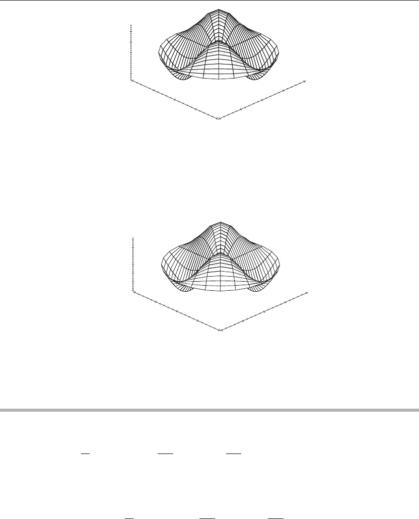
The preceding animation illustrates the spatial-time-dependent solution for u(r,θ,t). The
animation sequence in Figures 6.16 and 6.17 shows snapshots of the animation at the two
different times t = 0 and t = 4.
> u(r,theta,0):=subs(t=0,u(r,theta,t)):cylinderplot([r,theta,u(r,theta,0)],r=0..a,theta=−Pi..Pi,
axes=framed,thickness=1);

394 Chapter 6
0.2
0.1
0
20.1
21
20.5
21
20.5
0
0.5
20.2
0.5
0
11
z
y
x
Figure 6.16
> u(r,theta,4):=subs(t=4,u(r,theta,t)):cylinderplot([r,theta,u(r,theta,4)],r=0..a,theta=−Pi..Pi,
axes=framed,thickness=1);
0.02
0.03
0.01
0
20.01
20.02
20.03
z
21
20.5
21
20.5
0
0.5
0.5
0
11
y
x
Figure 6.17
Chapter Summary
Nonhomogeneous diffusion equation in two dimensions in rectangular coordinates
∂
∂t
u(x, y, t) = k
∂
2
∂x
2
u(x, y, t) +
∂
2
∂y
2
u(x, y, t)
+h(x, y, t)
Linear diffusion operator in two dimensions in rectangular coordinates
L(u) =
∂
∂t
u(x, y, t) −k
∂
2
∂x
2
u(x, y, t) +
∂
2
∂y
2
u(x, y, t)
Method of separation of variables solution
u(x, y, t) = X(x) Y(y) T(t)

The Diffusion Equation in Two Spatial Dimensions 395
Eigenfunction expansion solution for rectangular coordinates
u(x, y, t) =
∞
n=0
∞
m=0
X
m
(x) Y
n
(y) C(m, n)e
−kλ
m,n
t
Initial condition Fourier coefficients for rectangular coordinates
C(m, n) =
b
0
a
0
f(x, y)X
m
(x) Y
n
(y)dx dy
Nonhomogeneous diffusion equation in two dimensions in cylindrical coordinates
∂
∂t
u(r,θ,t)= k
⎛
⎝
∂
∂r
u(r,θ,t)+r
∂
2
∂r
2
u(r,θ,t)
r
+
∂
2
∂θ
2
u(r,θ,t)
r
2
⎞
⎠
+h(r,θ,t)
Linear diffusion operator in two dimensions in cylindrical coordinates
L(u) =
∂
∂t
u(r,θ,t)−k
⎛
⎝
∂
∂r
u(r,θ,t)+r
∂
2
∂r
2
u(r,θ,t)
r
+
∂
2
∂θ
2
u(r,θ,t)
r
2
⎞
⎠
Method of separation of variables solution
u(r,θ,t)= R(r)(θ)T(t)
Eigenfunction expansion solution in cylindrical coordinates
u(r,θ,t)=
∞
n=0
∞
m=0
R
m,n
(r)
m
(θ)C(m, n)e
−kλ
2
m,n
t
Initial condition Fourier coefficients for cylindrical coordinates
C(m, n) =
b
0
a
0
f(r, θ)R
m,n
(r)
m
(θ)rdr dθ
We have examined homogeneous partial differential equations describing diffusion phenomena
in two spatial dimensions for both the rectangular and the cylindrical coordinate systems.
Exercises
We now consider diffusion or heat equations with homogeneous boundary conditions in two
dimensions in both the rectangular coordinate and cylindrical coordinate systems. We use the
method of separation of variables and eigenfunction expansions to evaluate the solutions.

396 Chapter 6
Two Dimensions, Rectangular Coordinates
We seek the temperature distribution in thin plates over the two-dimensional domain
D ={(x, y) |0 <x<1, 0 <y<1} whose lateral surfaces are insulated. The two-dimensional
homogeneous partial differential equation in rectangular coordinates reads
∂
∂t
u(x, y, t) = k
∂
2
∂x
2
u(x, y, t) +
∂
2
∂y
2
u(x, y, t)
For Exercises 6.1 through 6.25, the initial condition u(x, y, 0) = f(x, y) and the boundary
conditions are given. You are asked to evaluate the eigenvalues and corresponding
two-dimensional orthonormal eigenfunctions and write the general solution. Generate the
animated three-dimensional surface solution u(x, y, t), and plot the animated sequence for
0 <t<5.
6.1. Boundaries x = 0,x= 1, y = 0,y= 1 are held at fixed temperature 0,k= 1/10:
u(0,y,t)= 0 and u(1,y,t)= 0
u(x, 0,t)= 0 and u(x, 1,t)= 0
Initial condition:
f(x, y) = x(1 −x) y(1 −y)
6.2. Boundaries x = 0,x= 2, y = 0 are held at fixed temperature 0, and boundary y = 1is
insulated, k = 1/10:
u(0,y,t)= 0 and u(2,y,t)= 0
u(x, 0,t)= 0 and u
y
(x, 1,t)= 0
Initial condition:
f(x, y) = x(2 −x)y
1 −
y
2
6.3. Boundaries x = 1,y= 0,y = 2 are held at fixed temperature 0, boundary x = 0is
insulated, k = 1/10:
u
x
(0,y,t)= 0 and u(1,y,t)= 0
u(x, 0,t)= 0 and u(x, 2,t)= 0
Initial condition:
f(x, y) = (1 −x
2
)y(2 −y)

The Diffusion Equation in Two Spatial Dimensions 397
6.4. Boundaries y = 0,y= 2 are held at fixed temperature 0, boundaries x = 0 and x = 1 are
insulated, k = 1/10:
u
x
(0,y,t)= 0 and u
x
(1,y,t)= 0
u(x, 0,t)= 0 and u(x, 2,t)= 0
Initial condition:
f(x, y) = x
2
1 −
2x
3
y(2 −y)
6.5. Boundaries x = 1,y = 1 are held at fixed temperature 0, boundaries x = 0 and y = 0 are
insulated, k = 1/10:
u
x
(0,y,t)= 0 and u(1,y,t)= 0
u
y
(x, 0,t)= 0 and u(x, 1,t)= 0
Initial condition:
f(x, y) = (1 −x
2
)(1 −y
2
)
6.6. Boundaries x = 1,y = 0 are held at fixed temperature 0, boundaries x = 0 and y = 1 are
insulated, k = 1/10:
u
x
(0,y,t)= 0 and u(1,y,t)= 0
u(x, 0,t)= 0 and u
y
(x, 1,t)= 0
Initial condition:
f(x, y) = (1 −x
2
)y
1 −
y
2
6.7. Boundary y = 0 is held at fixed temperature 0, boundaries x = 0, x = 1, and y = 1 are
insulated, k = 1/10:
u
x
(0,y,t)= 0 and u
x
(1,y,t)= 0
u(x, 0,t)= 0 and u
y
(x, 1,t)= 0
Initial condition:
f(x, y) = x
2
1 −
2x
3
y
1 −
y
2
