Articolo G.A. Partial Differential Equations and Boundary Value Problems with Maple V
Подождите немного. Документ загружается.


358 Chapter 6
This is the double Fourier series expansion of f(x, y). From Section 6.5, the Fourier
coefficients C(m, n) were evaluated by taking the double inner product of the initial condition
function f(x, y) with respect to the preceding corresponding orthonormalized eigenfunctions.
This yielded the double integral
> C(m,n):=eval(Int(Int(f(x,y)*X[m](x)*w(x)*Y[n](y)*w(y),x=0..a),y=0..b));C(m,0):=
expand(value(%)):
C(m, n) :=
1
0
1
0
2x(1 −x)y sin(mπx) cos(nπy)dx dy (6.31)
> C(m,n):=factor(subs({sin(m*Pi)=0,cos(m*Pi)=(−1)ˆm,sin(n*Pi)=0,cos(n*Pi)=(−1)ˆn},
C(m,n)));
C(m, n) := −
4(−1 +(−1)
n
)(−1 +(−1)
m
)
m
3
π
5
n
2
(6.32)
> C(m,0):=eval(Int(Int(f(x,y)*X[m](x)*w(x)*Y[0](y)*w(y),x=0..a),y=0..b));C(m,0):=
expand(value(%)):
C(m, 0) :=
1
0
1
0
x(1 −x)y
√
2 sin(mπx)dx dy (6.33)
> C(m,0):=simplify(subs({sin(m*Pi)=0,cos(m*Pi)=(−1)ˆm,sin(n*Pi)=0,cos(n*Pi)=(−1)ˆn},
C(m,0)));
C(m, 0) := −
√
2(−1 +(−1)
m
)
m
3
π
3
(6.34)
> T[m,n](t):=eval(T[m,n](t));
T
m,n
(t) := −
4(−1 +(−1)
n
)(−1 +(−1)
m
)e
−
1
50
(m
2
π
2
+n
2
π
2
)t
m
3
π
5
n
2
(6.35)
> T[m,0](t):=eval(T[m,0](t));
T
m,0
(t) := −
√
2(−1 +(−1)
m
)e
−
1
50
m
2
π
2
t
m
3
π
3
(6.36)
Generalized series terms for n = 0,m= 1, 2, 3,...,
> u[m,0](x,y,t):=eval(T[m,0](t)*X[m](x)*Y[0](y));
u
m,0
(x,y,t):= −
2(−1 +(−1)
m
)e
−
1
50
m
2
π
2
t
sin(mπx)
m
3
π
3
(6.37)

The Diffusion Equation in Two Spatial Dimensions 359
Generalized series terms for n = 1, 2, 3,...,m= 1, 2, 3,...,
> u[m,n](x,y,t):=eval(T[m,n](t)*X[m](x)*Y[n](y));
u
m,n
(x,y,t):= −
8(−1 +(−1)
n
)(−1 +(−1)
m
)e
−
1
50
(m
2
π
2
+n
2
π
2
)t
sin(mπx) cos(nπy)
m
3
π
5
n
2
(6.38)
Series solution
> u(x,y,t):=Sum(u[m,0](x,y,t),m=1..infinity)+Sum(Sum(u[m,n](x,y,t),m=1..infinity),
n=1..infinity);
u(x, y, t) :=
∞
m=1
⎛
⎝
−
2 (−1 +(−1)
m
)e
−
1
50
m
2
π
2
t
sin(mπx)
m
3
π
3
⎞
⎠
(6.39)
+
∞
n=1
⎛
⎝
∞
m=1
⎛
⎝
−
8(−1 +(−1)
n
)(−1 +(−1)
m
)e
−
1
50
(m
2
π
2
+n
2
π
2
)t
sin(mπx) cos(nπy)
m
3
π
5
n
2
⎞
⎠
⎞
⎠
First few terms of sum
> u(x,y,t):=sum(u[m,0](x,y,t),m=1..3)+sum(sum(u[m,n](x,y,t),m=1..3),n=1..3):
ANIMATION
> animate3d(u(x,y,t),x=0..a,y=0..b,t=0..5,axes=framed,thickness=1);
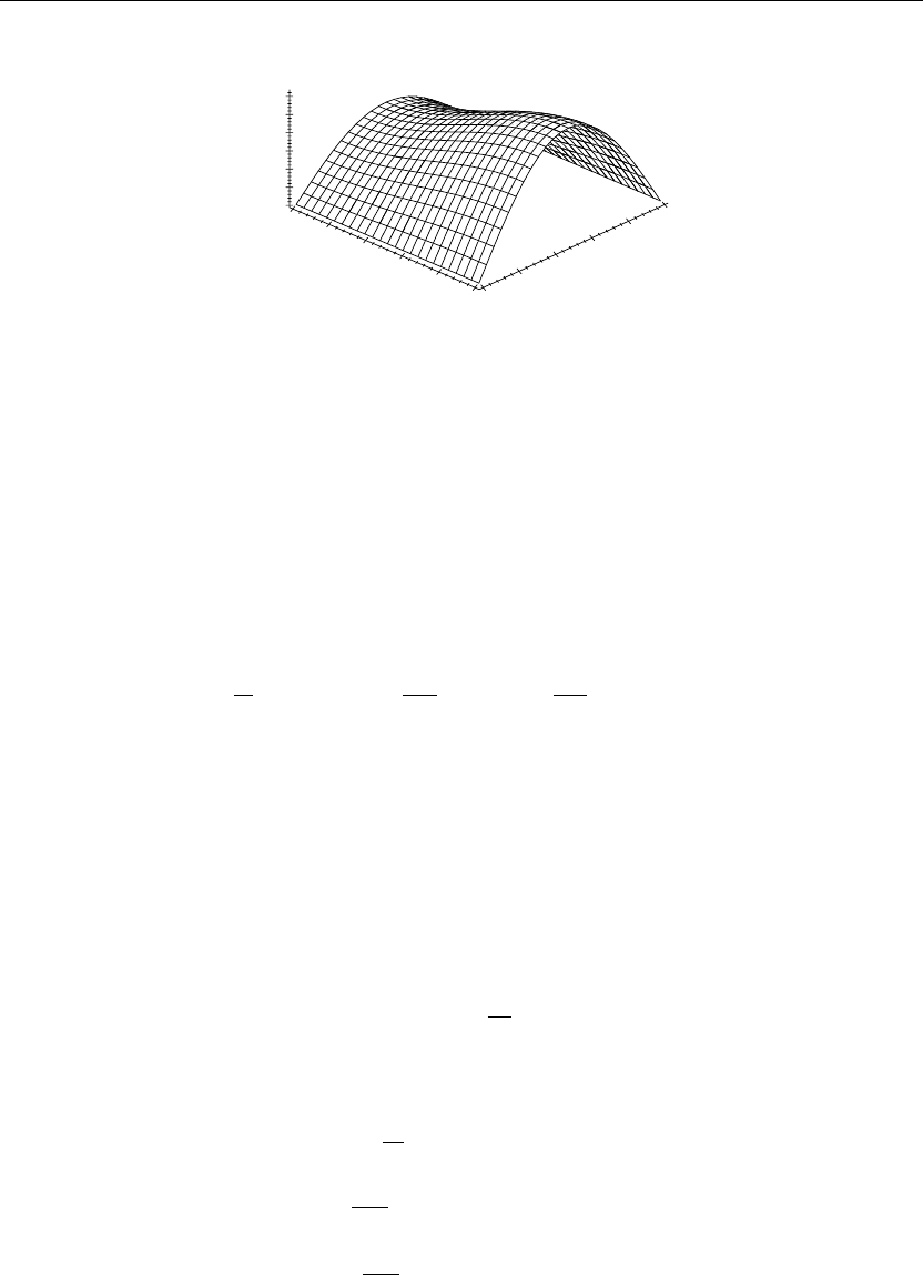
The preceding animation command illustrates the spatial-time-dependent solution for u(x, y, t).
The animation sequence in Figures 6.4 and 6.5 shows snapshots of the animation at two
different times t = 0 and t = 5.
ANIMATION SEQUENCE
> u(x,y,0):=subs(t=0,u(x,y,t)):plot3d(u(x,y,0),x=0..a,y=0..b,axes=framed,thickness=1);
x
y
1.0
0.8
0.6
0.4
0.2
0
1
0.8
0.6
0.4
0.2
0
0
0.05
0.15
0.1
0.2
Figure 6.4
360 Chapter 6
> u(x,y,5):=subs(t=5,u(x,y,t)):plot3d(u(x,y,5),x=0..a,y=0..b,axes=framed,thickness=1);
y
x
0.6
0.4
0.2
0.8
0
0.06
0.05
0.04
0.03
0.02
0.01
0
0
0.2
0.4
0.6
0.8
1
1
Figure 6.5
EXAMPLE 6.6.3: We seek the temperature distribution in a thin rectangular plate over the
finite two-dimensional domain D ={(x, y) |0 <x<1, 0 <y<1}. The lateral surfaces of the
plate are insulated. The boundaries y = 0 and y = 1 are fixed at temperature 0, the boundary
x = 0 is insulated, and the boundary x = 1 is losing heat by convection into a surrounding
medium at temperature 0. The initial temperature distribution f(x, y) is given as follows, and
the thermal diffusivity is k = 1/50.
SOLUTION: The two-dimensional homogeneous diffusion equation is
∂
∂t
u(x, y, t) = k
∂
2
∂x
2
u(x, y, t) +
∂
2
∂y
2
u(x, y, t)
The boundary conditions are type 2 at x =0, type 3 at x =1, type 1 at y = 0, and type 1 at y =1:
u
x
(0,y,t)= 0 and u
x
(1,y,t)+u(1,y,t)= 0
and
u(x, 0,t)= 0 and u(x, 1,t)= 0
The initial condition is
u(x, y, 0) =
1 −
x
2
3
y(1 −y)
The ordinary differential equations from the method of separation of variables are
d
dt
T(t) +kλT(t) = 0
d
2
dx
2
X(x)+αX(x)= 0
d
2
dy
2
Y(y) +βY(y)= 0

The Diffusion Equation in Two Spatial Dimensions 361
The coupling equation reads
λ = α +β
The boundary conditions on the spatial variables are
X
x
(0) = 0 and X
x
(1) +X(1) = 0
and
Y(0) = 0 and Y(1) = 0
Assignment of system parameters
> restart:with(plots):a:=1:b:=1:k:=1/50:
Allowed eigenvalues and corresponding orthonormal eigenfunctions are obtained from
Examples 2.5.1 and 2.5.5. Eigenvalues α
m
are the roots of the eigenvalue equation
> tan(sqrt(alpha[m])*a)=1/sqrt(alpha[m]);
tan
√
α
m
=
1
α
m
(6.40)
> beta[n]:=(n*Pi/b)ˆ2;lambda[m,n]:=alpha[m]+beta[n];
β
n
:= n
2
π
2
λ
m,n
:= α
m
+n
2
π
2
(6.41)
for m = 1, 2, 3,...,n= 1, 2, 3,....
Orthonormal eigenfunctions
> X[m](x):=sqrt(2)*(1/sqrt((sin(sqrt(alpha[m])*a)ˆ2+a)))*cos(sqrt(alpha[m])*x);X[r](x):=
subs(m=r,X[m](x)):
X
m
(x) :=
√
2 cos
√
α
m
x
sin
√
α
m
2
+1
(6.42)
> Y[n](y):=sqrt(2/b)*sin(n*Pi/b*y);Y[s](y):=subs(n=s,Y[n](y)):
Y
n
(y) :=
√
2 sin(nπy) (6.43)
Statements of orthonormality with their respective weight functions
> w(x):=1:Int(X[m](x)*X[r](x)*w(x),x=0..a)=delta(m,r);
1
0
2 cos
√
α
m
x
cos
√
α
r
x
sin
√
α
m
2
+1
sin
√
α
r
2
+1
dx = δ(m, r) (6.44)

362 Chapter 6
> w(y):=1:Int(Y[n](y)*Y[s](y)*w(y),y=0..b)=delta(n,s);
1
0
2 sin(nπy) sin(sπy)dy = δ(n, s) (6.45)
Time-dependent solution
> T[m,n](t):=C(m,n)*exp(−k*lambda[m,n]*t);
T
m,n
(t) := C(m, n)e
−
1
50
α
m
+n
2
π
2
t
(6.46)
Generalized series terms
> u[m,n](x,y,t):=T[m,n](t)*X[m](x)*Y[n](y);
u
m,n
(x,y,t):=
2C(m, n)e
−
1
50
α
m
+n
2
π
2
t
cos
√
α
m
x
sin(nπy)
sin
√
α
m
2
+1
(6.47)
Eigenfunction expansion
> u(x,y,t):=Sum(Sum(u[m,n](x,y,t),m=1..infinity),n=1..infinity);
u(x, y, t) :=
∞
n=1
⎛
⎜
⎝
∞
n=1
2C(m, n)e
−
1
50
α
m
+n
2
π
2
t
cos
√
α
m
x
sin(nπy)
sin
√
α
m
2
+1
⎞
⎟
⎠
(6.48)
The Fourier coefficients C(m, n) are to be determined from the initial condition function
u(x, y, 0) = f(x, y). We consider the special case
> f(x,y):=(1−xˆ2/3)*y*(1−y);
f(x, y) :=
1 −
1
3
x
2
y(1 −y) (6.49)
At time t = 0, we have
> f(x,y)=eval(subs(t=0,u(x,y,t)));
1 −
1
3
x
2
y(1 −y) =
∞
n=1
⎛
⎜
⎝
∞
m=1
2C(m, n) cos
√
α
m
x
sin (nπy)
sin
√
α
m
2
+1
⎞
⎟
⎠
(6.50)
This is the double Fourier series expansion of f(x, y). From Section 6.5, the Fourier
coefficients C(m, n) were evaluated by taking the double inner product of the initial condition
function f(x, y) with respect to the preceding corresponding orthonormalized eigenfunctions.
This yielded the double integral

The Diffusion Equation in Two Spatial Dimensions 363
> C(m,n):=eval(Int(Int(f(x,y)*X[m](x)*w(x)*Y[n](y)*w(y),x=0..a),y=0..b));C(m,n):=expand
(value(%)):
C (m, n) :=
1
0
1
0
2
1 −
1
3
x
2
y(1 −y) cos
√
α
m
x
sin(nπy)
sin
√
α
m
2
+1
dx dy (6.51)
> C(m,n):=radsimp(subs({sin(sqrt(alpha[m])*a)=1/sqrt(alpha[m])*cos(sqrt(alpha[m])*a),
sin(n*Pi)=0,cos(n*Pi)=(−1)ˆn},C(m,n)));
C(m, n) := −
8
3
cos
√
α
m
−1 +(−1)
n
α
2
m
n
3
π
3
2 −cos
√
α
m
2
(6.52)
> T[m,n](t):=eval(T[m,n](t));
T
m,n
(t) := −
8
3
cos
√
α
m
−1 +(−1)
n
e
−
1
50
α
m
+n
2
π
2
t
α
2
m
n
3
π
3
2 −cos
√
α
m
2
(6.53)
Generalized series terms
> u[m,n](x,y,t):=eval(T[m,n](t)*X[m](x)*Y[n](y));
u
m,n
(x,y,t):= −
16
3
cos
√
α
m
−1 +(−1)
n
e
−
1
50
α
m
+n
2
π
2
t
cos
√
α
m
x
sin (nπy)
α
2
m
n
3
π
3
2 −cos
√
α
m
2
sin
√
α
m
2
+1
(6.54)
Series solution
> u(x,y,t):=Sum(Sum(u[m,n](x,y,t),m=1..infinity),n=1..infinity);
u(x, y, t) :=
∞
n=1
⎛
⎜
⎝
∞
n=1
⎛
⎜
⎝
−
16
3
cos
√
α
m
−1 +(−1)
n
e
−
1
50
α
m
+n
2
π
2
t
cos
√
α
m
x
sin(nπy)
α
2
m
n
3
π
3
2 −cos
√
α
m
2
sin
√
α
m
2
+1
⎞
⎟
⎠
⎞
⎟
⎠
(6.55)
Evaluation of the eigenvalues α
m
from the roots of the eigenvalue equation yields
> tan(sqrt(alpha[m])*a)=1/sqrt(alpha[m]);
tan
√
α
m
=
1
√
α
m
(6.56)
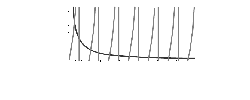
> plot({tab(v),1/v},v=0..20,y=0..3/2,thickness=10);
364 Chapter 6
0
0
0.5
y
v
1.0
1.5
5 101520
Figure 6.6
If we set v = a
√
α, then the eigenvalues α
m
are found from the squares of the values of v at the
intersection points of the curves shown in Figure 6.6. Using the Maple fsolve command to
evaluate the eigenvalues yields
> alpha[1]:=(1/aˆ2)*(fsolve((tan(v)−1/v),v=0..1)ˆ2);
α
1
:= 0.7401738844 (6.57)
> alpha[2]:=(1/aˆ2)*(fsolve((tan(v)−1/v),v=0..4)ˆ2);
α
2
:= 11.73486183 (6.58)
> alpha[3]:=(1/aˆ2)*(fsolve((tan(v)−1/v),v=4..7)ˆ2);
α
3
:= 41.43880785 (6.59)
First few terms of sum
> u(x,y,t):=eval(sum(sum(u[m,n](x,y,t),m=1..3),n=1..3)):
ANIMATION
> animate3d(u(x,y,t),x=0..a,y=0..b,t=0..5,axes=framed,thickness=1);
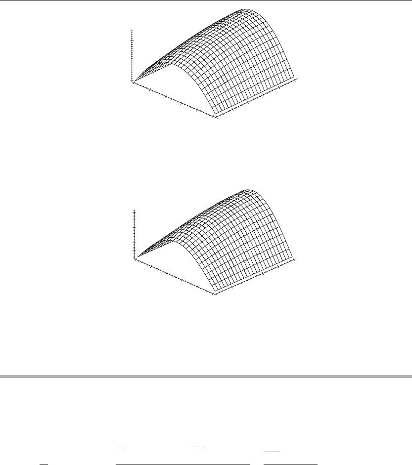
The preceding animation command illustrates the spatial-time-dependent solution for u(x, y, t).
The animation sequence in Figures 6.7 and 6.8 shows snapshots of the animation at the two
different times t = 0 and t = 3.
ANIMATION SEQUENCE
> u(x,y,0):=subs(t=0,u(x,y,t)):plot3d(u(x,y,0),x=0..a,y=0..b,axes=framed,thickness=1);
The Diffusion Equation in Two Spatial Dimensions 365
0.25
0.2
0.15
0.1
0.05
0
0
0.2
0.2
0
0.4
y
x
0.4
0.6
0.6
0.8
0.8
1
1
Figure 6.7
> u(x,y,3):=subs(t=3,u(x,y,t)):plot3d(u(x,y,3),x=0..a,y=0..b,axes=framed,thickness=1);
x
y
0.8
0.6
0.4
0.2
0
0.03
0.025
0.02
0.015
0.01
0.005
0
0
0.2
0.4
0.6
0.8
1
1
Figure 6.8
6.7 Diffusion Equation in the Cylindrical Coordinate
System
If we replace the preceding Laplacian operator in two dimensions from rectangular to
cylindrical coordinates, then the nonhomogeneous partial differential equation for diffusion or
heat phenomena in the cylindrical coordinate system in two dimensions is given as
∂
∂t
u(r,θ,t)= k
⎛
⎜
⎜
⎜
⎜
⎝
∂
∂r
u(r,θ,t)+r
∂
2
∂r
2
u(r,θ,t)
r
+
∂
2
∂θ
2
u(r,θ,t)
r
2
⎞
⎟
⎟
⎟
⎟
⎠
+h(r,θ,t)
where r is the coordinate radius of the system and θ is the polar angle. There is no z dependence
because we will only be considering very thin circular plates with no extension along the z-axis.
Similar to the rectangular coordinate system, we can write the preceding equation in terms of
the linear operator for the diffusion equation in cylindrical coordinates as
L(u) = h(r,θ,t)

366 Chapter 6
where the diffusion operator in cylindrical coordinates reads
L(u) =
∂
∂t
u(r,θ,t)−k
⎛
⎜
⎜
⎜
⎜
⎝
∂
∂r
u(r,θ,t)+
r
∂
2
∂r
2
u(r,θ,t)
r
+
∂
2
∂θ
2
u(r,θ,t)
r
2
⎞
⎟
⎟
⎟
⎟
⎠
Generally, one seeks a solution to this equation over the finite two-dimensional domain
D ={(r, θ) |0 <r<a,0 <θ<b} subject to the homogeneous boundary conditions
κ
1
u(a, θ, t) +κ
2
u
r
(a,θ,t)= 0
κ
3
u(r, 0,t)+κ
4
u
θ
(r, 0,t)= 0
κ
5
u(r,b,t)+κ
6
u
θ
(r,b,t)= 0
|
u(0,θ,t)
|
< ∞
along with the initial condition
u(r, θ, 0) = f(r, θ)
We now attempt to solve the homogeneous version [for no internal heat sources we set
h(r,θ,t)= 0] of this partial differential equation using the method of separation of variables.
We set
u(r,θ,t)= R(r) (θ) T(t)
Substituting this into the preceding homogeneous partial differential equation, we get
R(r)(θ)
d
dt
T(t)
=
k
⎛
⎜
⎜
⎜
⎜
⎝
d
dr
R(r)
(θ)T(t) +r
d
2
dr
2
R(r)
(θ)T(t)
r
+
R(r)
d
2
dθ
2
(θ)
T(t)
r
2
⎞
⎟
⎟
⎟
⎟
⎠
Dividing both sides by the product solution yields
d
dt
T(t)
kT(t)
=
(θ) r
d
dr
R(r)
+(θ) r
2
d
2
dr
2
R(r)
+R(r)
d
2
dθ
2
(θ)
R(r) (θ) r
2

The Diffusion Equation in Two Spatial Dimensions 367
Because the left-hand side of the preceding is an exclusive function of t and the right-hand side
an exclusive function of r and θ, and r, θ, and t are independent, the only way we can ensure
equality of the preceding for all values of r, θ, and t is to set each side equal to a constant.
Doing so, we arrive at the following three ordinary differential equations in terms of the
separation constants (for convenience here, we square the constants to ensure positivity).
d
dt
T(t) +kλ
2
T(t) = 0
d
2
dθ
2
(θ)+μ
2
(θ) = 0
r
2
d
2
dr
2
R(r)
+r
d
dr
R(r)
+
λ
2
r
2
−μ
2
R(r) = 0
The preceding differential equation in t is an ordinary first-order linear equation for which we
already have the solution from Chapter 1. The second differential equation in the variable θ is
recognized as being an Euler-type differential equation for which we generated solutions in
Section 1.4. The third differential equation is a Bessel-type differential equation whose
solutions are Bessel functions of the first kind of order μ as discussed in Section 1.11. We
recognize each of the two spatial differential equations in θ and r as being Sturm-Liouville-
type differential equations.
We first consider the second differential equation with respect to the variable θ subject to the
homogeneous boundary conditions over the finite interval I ={θ |0 <θ<b}. The
Sturm-Liouville problem for the θ-dependent portion of the diffusion equation consists of the
ordinary differential equation
d
2
dθ
2
(θ)+μ
2
(θ) = 0
along with the corresponding regular homogeneous boundary conditions, which read
κ
3
(0) +κ
4
θ
(0) = 0
and
κ
5
(b)+κ
6
θ
(b) = 0
We see the preceding problem in the variable θ to be a regular Sturm-Liouville eigenvalue
problem where the allowed values of μ are called the system “eigenvalues” and the
corresponding solutions are called the “eigenfunctions.” Note that this ordinary differential
equation is of the Euler type and the weight function is w(θ) = 1. The indexed eigenvalues and
corresponding eigenfunctions are given, respectively, as
μ
m
,
m
(θ)
for m = 0, 1, 2, 3,....
