Articolo G.A. Partial Differential Equations and Boundary Value Problems with Maple V
Подождите немного. Документ загружается.


248 Chapter 4
and
d
2
dr
2
R(r) +
d
dr
R(r)
r
+λ
2
R(r) = 0 (4.69)
We first consider the spatial differential equation in r. This is a Bessel-type differential
equation of the first kind of order zero with boundary conditions
|R(0)| < ∞ and R(1) = 0
This same problem was considered in Example 2.6.2 in Chapter 2. The allowed eigenvalues are
the roots of the eigenvalue equation
J(0,λ
n
) = 0
and the corresponding orthonormal eigenfunctions are
R
n
(r) =
√
2J(0,λ
n
r)
J(1,λ
n
)
for n = 1, 2, 3,....The functions J(0,λ
n
r) and J(1,λ
n
r) are Bessel functions of the first kind
of order zero and one, respectively.
The corresponding statement of orthonormality with respect to the weight function w(r) = r
over the interval I is
1
0
2J(0,λ
n
r)J(0,λ
m
r)r
J(1,λ
n
)J(1,λ
m
)
dr = δ(n, m)
for n = 1, 2, 3,..., and m = 1, 2, 3,....
We next consider the time-dependent differential equation. This is a second-order differential
equation that we solved in Section 1.4. The solution, for the allowed values of λ given
earlier, reads
T
n
(t) = e
−
t
5
(
A(n) cos
(
ω
n
t
)
+B(n) sin
(
ω
n
t
))
where
ω
n
=
λ
2
n
−1
5
Thus, the eigenfunction expansion solution to the problem reads
u(r, t) =
∞
n=1
e
−
t
5
(
A(n) cos
(
ω
n
t
)
+B(n) sin
(
ω
n
t
))
√
2J
(
0,λ
n
r
)
J(1,λ
n
)
The unknown coefficients A(n) and B(n) are to be determined from the initial conditions
imposed on the problem.

The Wave Partial Differential Equation 249
4.8 Initial Conditions for the Wave Equation in
Cylindrical Coordinates
We now consider the initial conditions on the problem. At time t = 0 we have the initial
displacement
u(r, 0) = f(r)
and the initial amplitude speed
u
t
(r, 0) = g(r)
Substituting the first condition into the general solution
u(r, t) =
∞
n=0
R
n
(r)e
−
γt
2
(
A(n) cos
(
ω
n
t
)
+B(n) sin
(
ω
n
t
))
at time t = 0 yields
f(r) =
∞
n=0
R
n
(r)A(n)
Substituting the second condition into the time derivative of the preceding at time t = 0 yields
g(r) =
∞
n=0
R
n
(r)
B(n)ω
n
−
A(n)γ
2
Because the eigenfunctions of this nonregular Sturm-Liouville problem form a complete set
with respect to piecewise smooth functions over the finite interval I ={r |a<r<b}, then
both of the preceding equations are the generalized Fourier series expansions of the functions
f(r) and g(r), respectively, in terms of the spatial eigenfunctions of the system. We now
evaluate the coefficients A(n) and B(n).
As we did in Section 2.3 for the generalized Fourier series expansion, we take the inner
product of both sides of the preceding equations, with respect to the weight function w(r) = r.
Operating on the first equation and using the statement of orthonormality, we get
b
a
f(r)R
m
(r)r dr =
∞
n=0
A(n)δ(n, m)
From the mathematical character of the Kronecker delta function, only one term (n = m)
survives in the preceding sum, and we are able to extract the value
A(m) =
b
a
f(r)R
m
(r)r dr

250 Chapter 4
In a similar manner, operating on the second equation and taking the inner product of both
sides and using the statement of orthonormality, we get
b
a
g(r)R
m
(r)r dr =
∞
n=0
B(n)ω
n
−
A(n)γ
2
δ(n, m)
Evaluating the sum (only the n = m term survives) and inserting the preceding known value
for A(m) yields
B(m) =
b
a
f(r)γ
2
+g(r)
R
m
(r)r dr
ω
m
Thus, we can write the final generalized solution to the wave equation in one dimension,
subject to the preceding homogeneous boundary and initial conditions, as
u(r, t) =
∞
n=0
R
n
(r)e
−
γt
2
⎛
⎜
⎜
⎜
⎜
⎜
⎜
⎜
⎝
⎛
⎝
b
a
f(r)R
n
(r)rdr
⎞
⎠
cos
(
ω
n
t
)
+
⎛
⎝
b
a
f(r)γ
2
+g(r)
R
n
(r)rdr
⎞
⎠
sin
(
ω
n
t
)
ω
n
⎞
⎟
⎟
⎟
⎟
⎟
⎟
⎟
⎠
(4.70)
All of the preceding operations are based on the assumption that the infinite series are
uniformly convergent, and the formal interchange between the operator and the summation is
legitimate. It can be shown that if the functions f(r) and g(r) satisfy the same boundary
conditions as the eigenfunctions, then the preceding series are, indeed, uniformly convergent.
DEMONSTRATION: We now provide a demonstration of these concepts for the example
problem given in Section 4.8 for the case where the initial conditions are
f(r) = 1 −r
2
and g(r) = 1 −r
2
SOLUTION: For the coefficient A(n), we have
A(n) =
1
0
(1 −r
2
)
√
2J(0,λ
n
r)r dr
J(1,λ
n
)
which evaluates to
A(n) =
4
√
2
λ
3
n

The Wave Partial Differential Equation 251
For the coefficient B(n), we have
B(n) =
1
0
6
√
2(1 −r)
2
J(0,λ
n
r)r dr
J(1,λ
n
)
λ
2
n
−1
which evaluates to
B(n) =
24
√
2
λ
3
n
λ
2
n
−1
for n = 1, 2, 3,....Thus, the final series solution to our problem reads
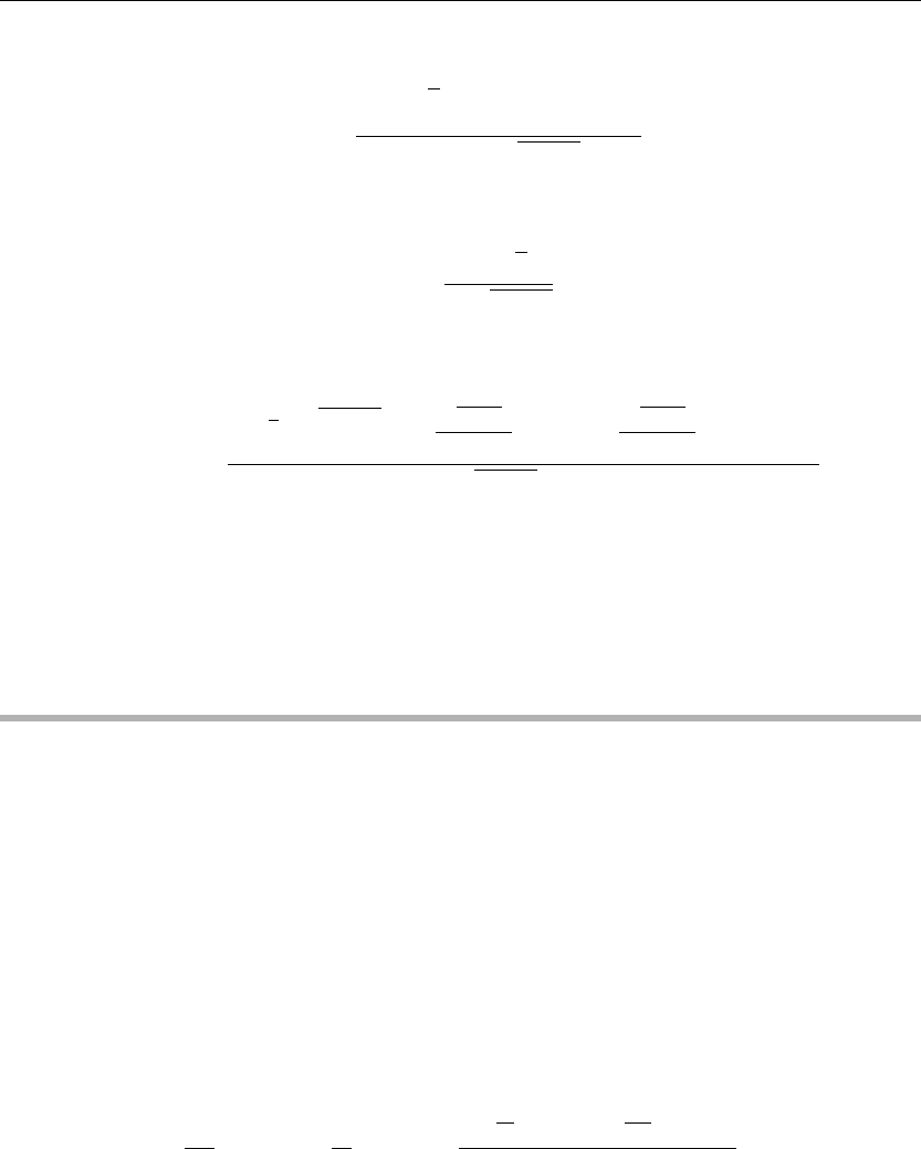
u(r, t) =
∞
n=1
8e
−
t
5
λ
2
n
−1 cos
√
λ
2
n
−1 t
5
+6 sin
√
λ
2
n
−1 t
5
J(0,λ
n
r)
λ
3
n
λ
2
n
−1J(1,λ
n
)
The detailed development of the solution to this problem and its graphics are given in one of
the Maple worksheet examples given later.
4.9 Example Wave Equation Problems in Cylindrical
Coordinates
We now consider several examples of partial differential equations for wave phenomena under
various homogeneous boundary conditions over finite intervals in the cylindrical coordinate
system. We note that all the spatial ordinary differential equations are of the Bessel type of
order zero and the weight function is w(r) = r.
EXAMPLE 4.9.1: We seek the wave distribution u(r, t) for transverse vibrations in a thin
circularly symmetric membrane over the interval I ={r |0 <r<1} that is secure at the
periphery. The membrane vibrates in a medium with a small amount of damping. The
membrane has an initial displacement distribution f(r) and an initial speed distribution g(r)
given as follows. The wave speed is c = 1/5, and the damping factor is γ = 2/5.
SOLUTION: The homogeneous wave equation is
∂
2
∂t
2
u(r, t) +γ
∂
∂t
u(r, t)
=
c
2
∂
∂r
u(r, t) +r
∂
2
∂r
2
u(r, t)
r
The boundary conditions are type 1 at r = 1 and a finite solution at r = 0
|u(0,t)| < ∞ and u(1,t)= 0

252 Chapter 4
The initial conditions are
u(r, 0) = 1 −r
2
and u
t
(r, 0) = 1 −r
2
The ordinary differential equations from the method of separation of variables are
d
2
dt
2
T(t) +γ
d
dt
T(t)
+c
2
λ
2
T(t) = 0
and
d
2
dr
2
R(r) +
d
dr
R(r)
r
+λ
2
R(r) = 0 (4.71)
The boundary conditions on the spatial equation are
|R(0)| < ∞ and R(1) = 0
Assignment of system parameters
> restart:with(plots):a:=0:b:=1:c:=1/5:unprotect(gamma):gamma:=2/5:
Allowed eigenvalues and orthonormalized eigenfunctions are obtained from Example 2.6.2.
The eigenvalues are the roots of the eigenvalue equation
> BesselJ(0,lambda[n]*b)=0;
BesselJ
(
0,λ
n
)
= 0 (4.72)
for n = 1, 2, 3,....
> R[n](r):=simplify(BesselJ(0,lambda[n]*r)/sqrt(int(BesselJ(0,lambda[n]*r)ˆ2*r,r=a..b)));
R
n
(r) :=
BesselJ(0,λ
n
r)
√
2
BesselJ(0,λ
n
)
2
+ BesselJ(1,λ
n
)
2
(4.73)
Substitution of the eigenvalue equation simplifies the preceding equation
> R[n](r):=radsimp(subs(BesselJ(0,lambda[n]*b)=0,R[n](r)));R[m](r):=subs(n=m,R[n](r)):
R
n
(r) :=
BesselJ(0,λ
n
r)
√
2
BesselJ(1,λ
n
)
(4.74)
Statement of orthonormality with respect to the weight function w(r) = 1
> w(r):=r:Int(R[n](r)*R[m](r)*w(r),r=a..b)=delta(n,m);
1
0
2 BesselJ(0,λ
n
r)BesselJ(0,λ
m
r)r
BesselJ(1,λ
n
)BesselJ(1,λ
m
)
dr = δ(n, m) (4.75)

The Wave Partial Differential Equation 253
Time-dependent solution
> T[n](t):=exp((−gamma/2)*t)*(A(n)*cos(omega[n]*t)+B(n)*sin(omega[n]*t));
T
n
(t) := e
−
1
5
t
(
A(n) cos
(
ω
n
t
)
+B(n) sin
(
ω
n
t
))
(4.76)
Generalized series terms
> u[n](r,t):=T[n](t)*R[n](r):
Eigenfunction expansion
> u(r,t):=Sum(u[n](r,t),n=1..infinity);
u(r, t) :=
∞
n=1
e
−
1
5
t
(
A(n) cos
(
ω
n
t
)
+B(n) sin
(
ω
n
t
))
BesselJ
(
0,λ
n
r
)
√
2
BesselJ
(
1,λ
n
)
(4.77)
> omega[n]:=sqrt(lambda[n]ˆ2*cˆ2−gammaˆ2/4);
ω
n
:=
1
5
λ
2
n
−1 (4.78)
From Section 4.8, the coefficients A(n) and B(n) are to be determined from the inner product
of the eigenfunctions and the initial condition functions u(r, 0) = f(r) and u
t
(r, 0) = g(r).
> f(r):=1−rˆ2;
f(r) := 1 −r
2
(4.79)
> g(r):=1−rˆ2;
g(r) := 1 −r
2
(4.80)
For n = 1, 2, 3,...,
> A(n):=eval(Int(f(r)*R[n](r)*w(r),r=a..b));A(n):=value(%):
A(n) :=
1
0
(1 −r
2
) BesselJ(0,λ
n
r)
√
2 r
BesselJ(1,λ
n
)
dr (4.81)
Substitution of the eigenvalue equation simplifies the preceding equation
> A(n):=simplify(subs(BesselJ(0,lambda[n]*b)=0,A(n)));
A(n) :=
4
√
2
λ
3
n
(4.82)

254 Chapter 4
> B(n):=eval(Int((f(r)*gamma/2+g(r))*R[n](r)*w(r),r=a..b))/omega[n];B(n):=value(%):
B(n) :=
5
⎛
⎝
1
0
6
5
−
6
5
r
2
BesselJ(0,λ
n
r)
√
2r
BesselJ(1,λ
n
)
dr
⎞
⎠
λ
2
n
−1
(4.83)
Substitution of the eigenvalue equation simplifies the preceding equation
> B(n):=simplify(subs(BesselJ(0,lambda[n]*b)=0,B(n)));
B(n) :=
24
√
2
λ
3
n
λ
2
n
−1
(4.84)
Generalized series terms
> u[n](r,t):=simplify(eval(T[n](t)*R[n](r))):
Series solution
> u(r,t):=Sum(u[n](r,t),n=1..infinity);
u(r, t) :=
∞
n=1
8e
−
1
5
t
BesselJ(0,λ
n
r)
cos
1
5
λ
2
n
−1 t
λ
2
n
−1 +6 sin
1
5
λ
2
n
−1 t
BesselJ(1,λ
n
)λ
3
n
λ
2
n
−1
(4.85)
Evaluation of the eigenvalues from the roots of the eigenvalue equation yields
> BesselJ(0,lambda[n]*b)=0;
BesselJ(0,λ
n
) = 0 (4.86)
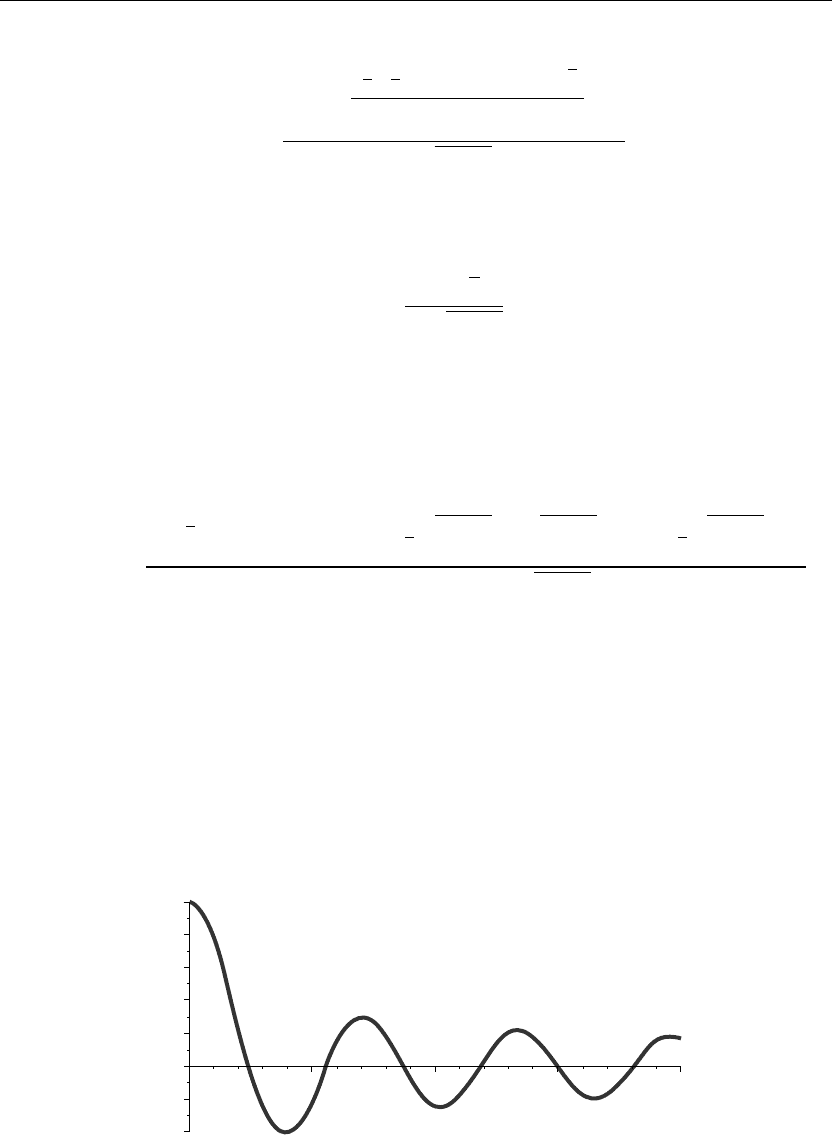
> plot(BesselJ(0,v),v=0..20,thickness=10);
If we set v = λb, then the eigenvalues are determined from the intersection points of the curve
with the v-axis shown in Figure 4.7. Evaluation of a few of the eigenvalues using the Maple
fsolve command yields
10 15 20
20.4
20.2
0
0.2
0.4
0.6
0.8
1.0
5
v
Figure 4.7

The Wave Partial Differential Equation 255
> lambda[1]:=(1/b)*fsolve(BesselJ(0,v)=0,v=0..3);
λ
1
:= 2.404825558 (4.87)
> lambda[2]:=(1/b)*fsolve(BesselJ(0,v)=0,v=3..6);
λ
2
:= 5.520078110 (4.88)
> lambda[3]:=(1/b)*fsolve(BesselJ(0,v)=0,v=6..9);
λ
3
:= 8.653727913 (4.89)
First few terms in sum
> u(r,t):=eval(sum(u[n](r,t),n=1..3)):
ANIMATION
> animate(u(r,t),r=a..b,t=0..2,thickness=3);
The preceding animation command illustrates the spatial-time-dependent solution for u(r, t).
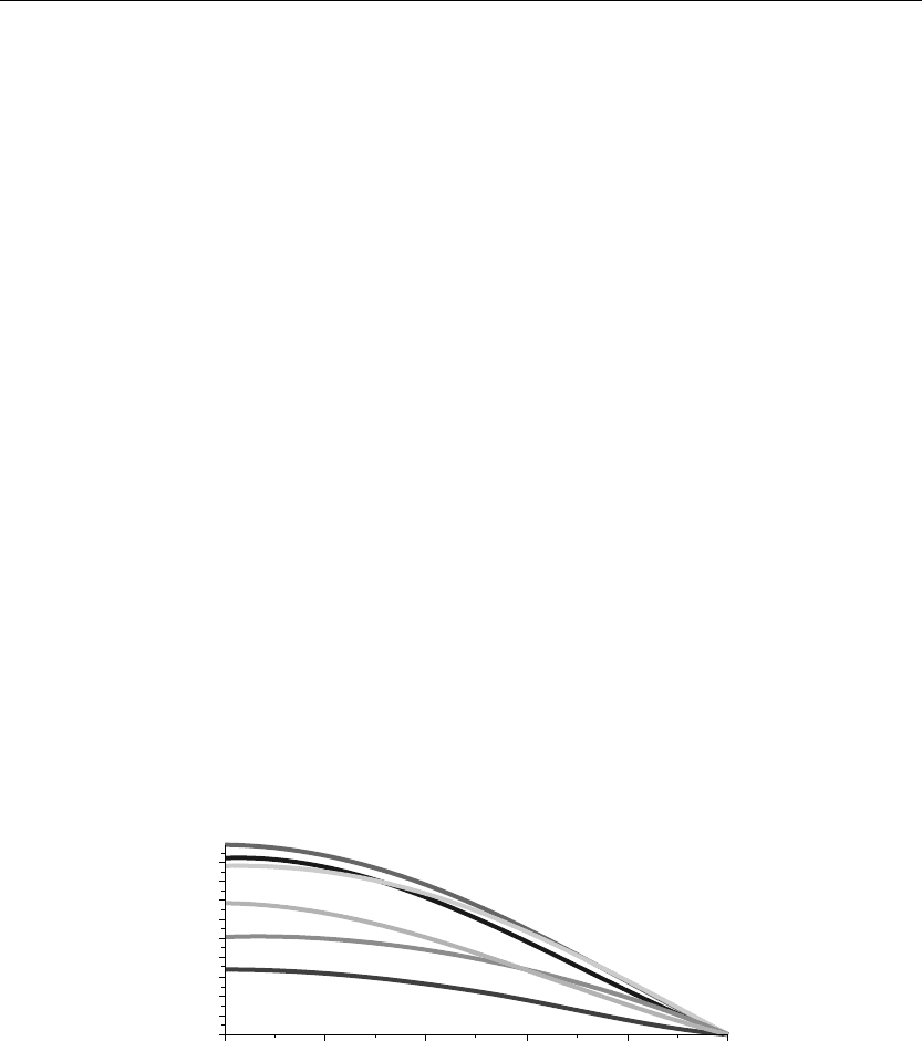
The following animation sequence in Figure 4.8 shows snapshots of the animation at times
t = 0, 1, 2, 3, 4, and 5.
ANIMATION SEQUENCE
> u(r,0):=subs(t=0,u(r,t)):u(r,1):=subs(t=1,u(r,t)):
> u(r,2):=subs(t=2,u(r,t)):u(r,3):=subs(t=3,u(r,t)):
> u(r,4):=subs(t=4,u(r,t)):u(r,5):=subs(t=5,u(r,t)):
> plot({u(r,0),u(r,1),u(r,2),u(r,3),u(r,4),u(r,5)},r=a..b,thickness=10);
r
0 0.2 0.4 0.6 0.8 1
0
0.6
1
1.4
1.8
Figure 4.8
THREE-DIMENSIONAL ANIMATION
> u(x,y,t):=eval(subs(r=sqrt(xˆ2+yˆ2),u(r,t))):
> u(x,y,t):=(u(x,y,t))*Heaviside(1−sqrt(xˆ2+yˆ2)):
> animate3d(u(x,y,t),x=−b..b,y=−b..b,t=0..10,axes=framed,thickness=1);

256 Chapter 4
EXAMPLE 4.9.2: We consider transverse vibrations in a thin circularly symmetric membrane
over the interval I ={r |0 <r<1}, which is unsecured at the periphery. The membrane
vibrates in a medium with very small damping. The membrane has an initial displacement
distribution f(r) and an initial speed distribution g(r) given as follows. The wave speed is
c = 1/5, and the damping factor is γ = 2/5.
SOLUTION: The homogeneous wave equation is
∂
2
∂t
2
u(r, t) +γ
∂
∂t
u(r, t)
=
c
2
∂
∂r
u(r, t) +r
∂
2
∂r
2
u(r, t)
r
The boundary conditions are type 2 at r = 1 and a finite solution at r = 0
|u(0,t)| < ∞ and u
r
(1,t)= 0
The initial conditions are
u(r, 0) = 1 −r
2
and u
t
(r, 0) = 1 −r
2
The ordinary differential equations from the method of separation of variables are
d
2
dt
2
T(t) +γ
d
dt
T(t)
+c
2
λ
2
T(t) = 0
and
d
2
dr
2
R(r) +
d
dr
R(r)
r
+λ
2
R(r) = 0 (4.90)
The boundary conditions on the spatial equation are
|R(0)| < ∞ and R
r
(1) = 0
Assignment of system parameters
> restart:with(plots):a:=0:b:=1:c:=1/5:unprotect(gamma):gamma:=2/5:
Allowed eigenvalues and orthonormalized eigenfunctions are obtained from Example 2.6.3.
> lambda[0]:=0;
λ
0
:= 0 (4.91)
for n = 0.
> R[0](r):=sqrt(2)/b;
R
0
(r) :=
√
2 (4.92)
For n = 1, 2, 3,..., the eigenvalues are the roots of the eigenvalue equation

The Wave Partial Differential Equation 257
> subs(r=b,diff(BesselJ(0,lambda[n]*r),r)=0);
−BesselJ(1,λ
n
)λ
n
= 0 (4.93)
> R[n](r):=simplify(BesselJ(0,lambda[n]*r)/sqrt(int(BesselJ(0,lambda[n]*r)ˆ2*r,r=a..b)));
R
n
(r) :=
BesselJ(0,λ
n
r)
√
2
BesselJ(0,λ
n
)
2
+ BesselJ(1,λ
n
)
2
(4.94)
Substitution of the eigenvalue equation simplifies the preceding equation
> R[n](r):=radsimp(subs(BesselJ(1,lambda[n]*b)=0,R[n](r)));R[m](r):=subs(n=m,R[n](r)):
R
n
(r) :=
BesselJ(0,λ
n
r)
√
2
BesselJ(0,λ
n
)
(4.95)
Statement of orthonormality with respect to the weight function w(r) = r
> w(r):=r:Int(R[n](r)*R[m](r)*w(r),r=a..b)=delta(n,m);
1
0
2 BesselJ(0,λ
n
r) BesselJ(0,λ
m
r)r
BesselJ(0,λ
n
) BesselJ(0,λ
m
)
dr = δ(n, m) (4.96)
Time-dependent solution
> T[0](t):=A(0)+B(0)*exp(−gamma*t);
T
0
(t) := A(0) +B(0)e
−
2
5
t
(4.97)
for n = 0.
> T[n](t):=exp((−gamma/2)*t)*(A(n)*cos(omega[n]*t)+B(n)*sin(omega[n]*t));
T
n
(t) := e
−
1
5
t
(
A(n) cos
(
ω
n
t
)
+B(n) sin
(
ω
n
t
))
(4.98)
for n = 1, 2, 3,....
Generalized series terms
> u[0](r,t):=eval(T[0](t)*R[0](r)):u[n](r,t):=eval(T[n](t)*R[n](r)):
Eigenfunction expansion
> u(r,t):=u[0](r,t)+Sum(u[n](r,t),n=1..infinity);
u(r, t) :=
A(0) +B(0)e
−
2
5
t
√
2
+
∞
n=1
e
−
1
5
t
(
A(n) cos
(
ω
n
t
)
+B(n) sin
(
ω
n
t
))
BesselJ(0,λ
n
r)
√
2
BesselJ(0,λ
n
)
(4.99)
