Articolo G.A. Partial Differential Equations and Boundary Value Problems with Maple V
Подождите немного. Документ загружается.


178 Chapter 3
For n = 0,
> T[0](t):=eval(subs(n=0,T[n](t)));u[0](x,t):=T[0](t)*X[0](x):
T
0
(t) := C(0) (3.29)
Eigenfunction expansion
> u(x,t):=u[0](x,t)+Sum(u[n](x,t),n=1..infinity);
u(x, t) := C(0) +
∞
n=1
C(n)e
−
1
10
n
2
π
2
t
√
2 cos(nπx) (3.30)
Evaluation of Fourier coefficients for the specific initial condition
> f(x):=x;
f(x) := x (3.31)
> C(n):=Int(f(x)*X[n](x)*w(x),x=a..b);C(n):=expand(value(%)):
C(n) :=
1
0
x
√
2 cos(nπx) dx (3.32)
> C(n):=radsimp(subs({sin(n*Pi)=0,cos(n*Pi)=(−1)ˆn},C(n)));
C(n) :=
√
2(−1 +(−1)
n
)
n
2
π
2
(3.33)
> C(0):=Int(f(x)*X[0](x)*w(x),x=a..b);C(0):=expand(value(%)):
C(0) :=
1
0
x dx (3.34)
> C(0):=value(%);
C(0) :=
1
2
(3.35)
> u[0](x,t):=eval(T[0](t)*X[0](x));
Generalized series terms
> u[n](x,t):=eval(T[n](t)*X[n](x));
u
n
(x, t) :=
2(−1 +(−1)
n
) e
−
1
10
n
2
π
2
t
cos(nπx)
n
2
π
2
(3.36)

The Diffusion or Heat Partial Differential Equation 179
Series solution
> u(x,t):=eval(u[0](x,t)+Sum(u[n](x,t),n=1..infinity));
u(x, t) :=
1
2
+
∞
n=1
2(−1 +(−1)
n
)e
−
1
10
n
2
π
2
t
cos(nπx)
n
2
π
2
(3.37)
First few terms of sum
> u(x,t):=eval(u[0](x,t)+sum(u[n](x,t),n=1..3)):
ANIMATION
> animate(u(x,t),x=a..b,t=0..4,color=red,thickness=3);
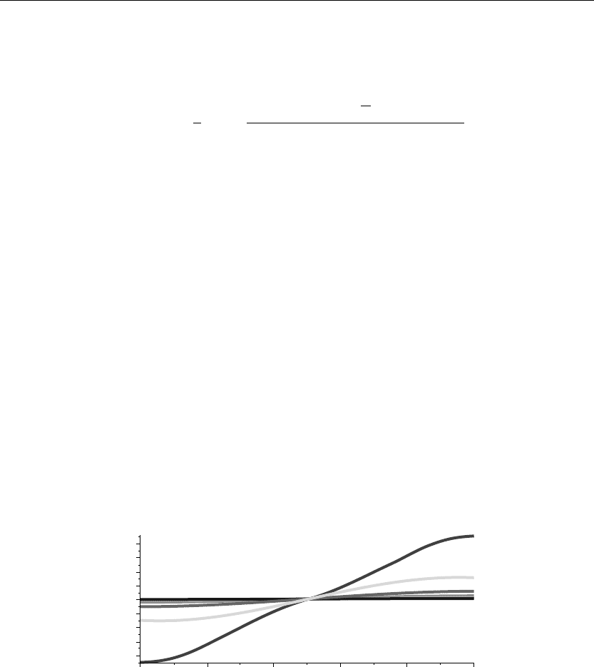
The preceding animation command illustrates the spatial-time-dependent solution for u(x, t).
The animation sequence shown in Figure 3.3 shows snapshots at times t = 0, 1, 2, 3, 4, and 5.
ANIMATION SEQUENCE
> u(x,0):=subs(t=0,u(x,t)):u(x,1):=subs(t=1,u(x,t)):
> u(x,2):=subs(t=2,u(x,t)):u(x,3):=subs(t=3,u(x,t)):
> u(x,4):=subs(t=4,u(x,t)):u(x,5):=subs(t=5,u(x,t)):
> plot({u(x,0),u(x,1),u(x,2),u(x,3),u(x,4),u(x,5),},x=a..b,thickness=10);
0.1
0.2
0.3
0.4
0.5
0.6
0.7
0.8
0.9
x
0 0.2 0.4 0.6 0.8 1
Figure 3.3
EXAMPLE 3.6.4: We consider the temperature distribution u(x, t) in a thin rod whose lateral
surface is insulated over the finite interval I ={x |0 <x<1}. The left end of the rod is
insulated and the right end experiences a convection heat loss. The initial temperature
distribution f(x) is given following, and the diffusivity is k = 1/5.

180 Chapter 3
SOLUTION: The homogeneous diffusion equation is
∂
∂t
u(x, t) = k
∂
2
∂x
2
u(x, t)
The boundary conditions are type 2 at x = 0 and type 3 at x = 1
u
x
(0,t)= 0 and u
x
(1,t)+u(1,t)= 0
The initial condition is
u(x, 0) = 1 −
x
3
4
Ordinary differential equations obtained from the method of separation of variables:
d
dt
T(t) +kλT(t) = 0
and
d
2
dx
2
X(x)+λX(x) = 0
Boundary conditions on spatial equation
X
x
(0) = 0 and X
x
(1) +X(1) = 0
Assignment of system parameters
> restart:with(plots):a:=0:b:=1:k:=1/5:
Allowed eigenvalues and orthonormal eigenfunctions are obtained from Example 2.5.5. The
eigenvalues are the roots of the eigenvalue equation
> tan(sqrt(lambda[n])*b)=1/sqrt(lambda[n]);
tan
λ
n
=
1
√
λ
n
(3.38)
for n = 1, 2, 3,....
Orthonormal eigenfunctions
> X[n](x):=sqrt(2)*cos(sqrt(lambda[n])*x)/sqrt(((sin(sqrt(lambda[n])*b))ˆ2+b));
X[m](x):=subs(n=m,X[n](x)):
X
n
(x) :=
√
2 cos
√
λ
n
x
sin
√
λ
n
2
+1
(3.39)

The Diffusion or Heat Partial Differential Equation 181
Statement of orthonormality with respect to the weight function w(x) = 1
> w(x):=1:Int(X[n](x)*X[m](x)*w(x),x=a...b)=delta(n,m);
1
0
2 cos
√
λ
n
x
cos
√
λ
m
x
sin
√
λ
n
2
+1
√
λ
m
2
+1
dx = δ(n, m) (3.40)
Time-dependent solution
> T[n](t):=C(n)*exp(−k*lambda[n]*t);u[n](x,t):=T[n](t)*X[n](x):
T
n
(t) := C(n)e
−
1
5
λ
n
t
(3.41)
Generalized series terms
> u[n](x,t):=T[n](t)*X[n](x);
u
n
(x, t) :=
C(n)e
−
1
5
λ
n
t
√
2 cos
√
λ
n
x
sin
√
λ
n
2
+1
(3.42)
Eigenfunction expansion
> u(x,t):=Sum(u[n](x,t),n=1..infinity);
u(x, t) :=
∞
n=1
C(n)e
−
1
5
λ
n
t
√
2 cos
√
λ
n
x
sin
√
λ
n
2
+1
(3.43)
Evaluation of Fourier coefficients for the specific initial condition
> f(x):=1−xˆ3/4;
f(x) := 1 −
1
4
x
3
(3.44)
> C(n):=Int(f(x)*X[n](x)*w(x),x=a..b);C(n):=simplify(value(%)):
C(n) :=
1
0
1 −
1
4
x
3
√
2 cos
√
λ
n
x
sin
√
λ
n
2
+1
dx (3.45)
Substitution of the eigenvalue equation simplifies this integral

182 Chapter 3
> C(n):=simplify(subs(sin(sqrt(lambda[n])*b)=(1/sqrt(lambda[n]))*cos(sqrt(lambda[n])*b),
C(n)));
C(n) :=
3
2
√
2
−1 +2 cos
√
λ
n
λ
2
n
2 −cos
√
λ
n
2
(3.46)
Generalized series terms
> u[n](x,t):=eval(T[n](t)*X[n](x));
u
n
(x, t) :=
3
−1 +2 cos
√
λ
n
e
−
1
5
λ
n
t
cos
√
λ
n
x
λ
2
n
2 −cos
√
λ
n
2
sin
√
λ
n
2
+1
(3.47)
Series solution
> u(x,t):=Sum(u[n](x,t),n=1..infinity);
u(x, t) :=
∞
n=1
3
−1 +2 cos
√
λ
n
e
−
1
5
λ
n
t
cos
√
λ
n
x
λ
2
n
2 −cos
√
λ
n
2
sin
√
λ
n
2
+1
(3.48)
Evaluation of the eigenvalues from the roots of the eigenvalue equation yields
> tan(sqrt(lambda[n]*b))=1/sqrt(lambda[n]);
tan
λ
n
=
1
√
λ
n
(3.49)
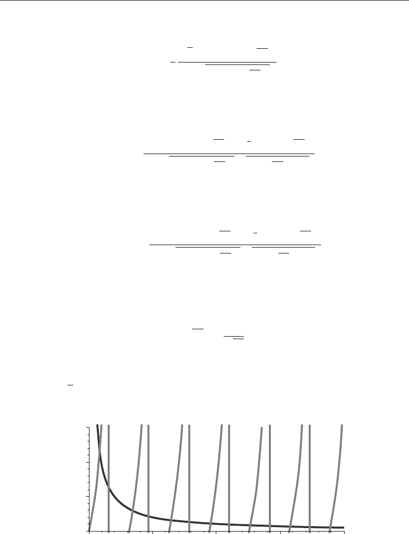
> plot({tan(v),1/v},v=0..20,y=0..3/2,thickness=10);
If we set v =
√
λb, then the eigenvalues are found from the intersection points of the curves
shown in Figure 3.4. We evaluate a few of these eigenvalues using the Maple fsolve command:
0
0.5
1.0
1.5
0 5 10 15 20
y
v
Figure 3.4

The Diffusion or Heat Partial Differential Equation 183
> lambda[1]:=(1/b*(fsolve((tan(v)−1/v),v=0..1)))ˆ2;
λ
1
:= 0.7401738844 (3.50)
> lambda[2]:=(1/b*(fsolve((tan(v)−1/v),v=1..4)))ˆ2;
λ
2
:= 11.73486183 (3.51)
> lambda[3]:=(1/b*(fsolve((tan(v)−1/v),v=4..7)))ˆ2;
λ
3
:= 41.43880785 (3.52)
First few terms of sum
> u(x,t):=eval(sum(u[n](x,t),n=1..3)):
ANIMATION
> animate(u(x,t),x=a..b,t=0..10,thickness=10);
The preceding animation command illustrates the spatial-time-dependent solution for u(x, t).
The animation sequence shown in Figure 3.5 shows snapshots at times t = 0, 1, 2, 3, 4, and 5.
ANIMATION SEQUENCE
> u(x,0):=subs(t=0,u(x,t)):u(x,1):=subs(t=1,u(x,t)):
> u(x,2):=subs(t=2,u(x,t)):u(x,3):=subs(t=3,u(x,t)):
> u(x,4):=subs(t=4,u(x,t)):u(x,5):=subs(t=5,u(x,t)):
0.4
0.5
0.6
0.7
0.8
0.9
1.0
0 0.2 0.4 0.6 0.8 1
x
Figure 3.5
EXAMPLE 3.6.5: We seek the temperature distribution u(x, t) in a thin rod over the finite
interval I ={x |0 <x<1}. This rod experiences heat loss through the lateral surface into a
surrounding medium of temperature zero. The coefficient β accounts for the heat loss. Both the
left and right ends of the rod are held at the fixed temperature zero. The initial temperature
distribution f(x) is given following, β = 1/5, and the diffusivity is k = 1/10.

184 Chapter 3
SOLUTION: The homogeneous diffusion equation is
∂
∂t
u(x, t) = k
∂
2
∂x
2
u(x, t)
−βu(x, t) (3.53)
The boundary conditions are type 1 at x = 0 and type 1 at x = 1
u(0,t)= 0 and u(1,t)= 0
The initial condition is
u(x, 0) = x(1 −x)
Ordinary differential equations obtained from the method of separation of variables
d
dt
T(t) +kλT(t) = 0
and
d
2
dx
2
X(x)+
λ −
β
k
X(x) = 0
Boundary conditions on spatial equation
X(0) = 0 and X(1) = 0
Assignment of system parameters
> restart:with(plots):a:=0:b:=1:k:=1/10:beta:=1/5:
Allowed eigenvalues and orthonormal eigenfunctions are obtained from Example 2.5.1.
> lambda[n]:=(n*Pi/b)ˆ2+beta/k;
λ
n
:= n
2
π
2
+2 (3.54)
for n = 1, 2, 3,....
Orthonormal eigenfunctions
> X[n](x):=sqrt(2/b)*sin(n*Pi/b*x);X[m](x):=subs(n=m,X[n](x)):
X
n
(x) :=
√
2 sin(nπx) (3.55)
Statement of orthonormality with respect to the weight function w(x) = 1
> w(x):=1:Int(X[n](x)*X[m](x)*w(x),x=a...b)=delta(n,m);
1
0
2 sin(nπx) sin(mπx)dx = δ(n, m) (3.56)

The Diffusion or Heat Partial Differential Equation 185
Time-dependent solution
> T[n](t):=C(n)*exp(−k*lambda[n]*t);
T
n
(t) := C(n)e
−
1
10
(n
2
π
2
+2)t
(3.57)
Generalized series terms
> u[n](x,t):=T[n](t)*X[n](x);
u
n
(x, t) := C(n)e
−
1
10
(n
2
π
2
+2)t
√
2 sin(nπx) (3.58)
Eigenfunction expansion
> u(x,t):=Sum(u[n](x,t),n=1..infinity);
u(x, t) :=
∞
n=1
C(n)e
−
1
10
(n
2
π
2
+2)t
√
2 sin(nπx) (3.59)
Evaluation of Fourier coefficients for the specific initial condition
> f(x):=x*(1−x);
f(x) := x(1 −x) (3.60)
> C(n):=Int(f(x)*X[n](x)*w(x),x=a..b);C(n):=expand(value(%)):
C(n) :=
1
0
x(1 −x)
√
2 sin(nπx) dx (3.61)
> C(n):=simplify(subs({sin(n*Pi)=0,cos(n*Pi)=(−1)ˆn},C(n)));
C(n) := −
2
√
2(−1 +(−1)
n
)
n
3
π
3
(3.62)
Generalized series terms
> u[n](x,t):=eval(T[n](t)*X[n](x));
u
n
(x, t) := −
4(−1 +(−1)
n
)e
−
1
10
n
2
π
2
+2
t
sin(nπx)
n
3
π
3
(3.63)
Series solution
> u(x,t):=Sum(u[n](x,t),n=1..infinity);
u(x, t) :=
∞
n=1
−
4(−1 +(−1)
n
)e
−
1
10
(n
2
π
2
+2)t
sin(nπx)
n
3
π
3
(3.64)

186 Chapter 3
First few terms of sum
> u(x,t):=sum(u[n](x,t),n=1..3):
ANIMATION
> animate(u(x,t),x=a..b,t=0..5,thickness=3);
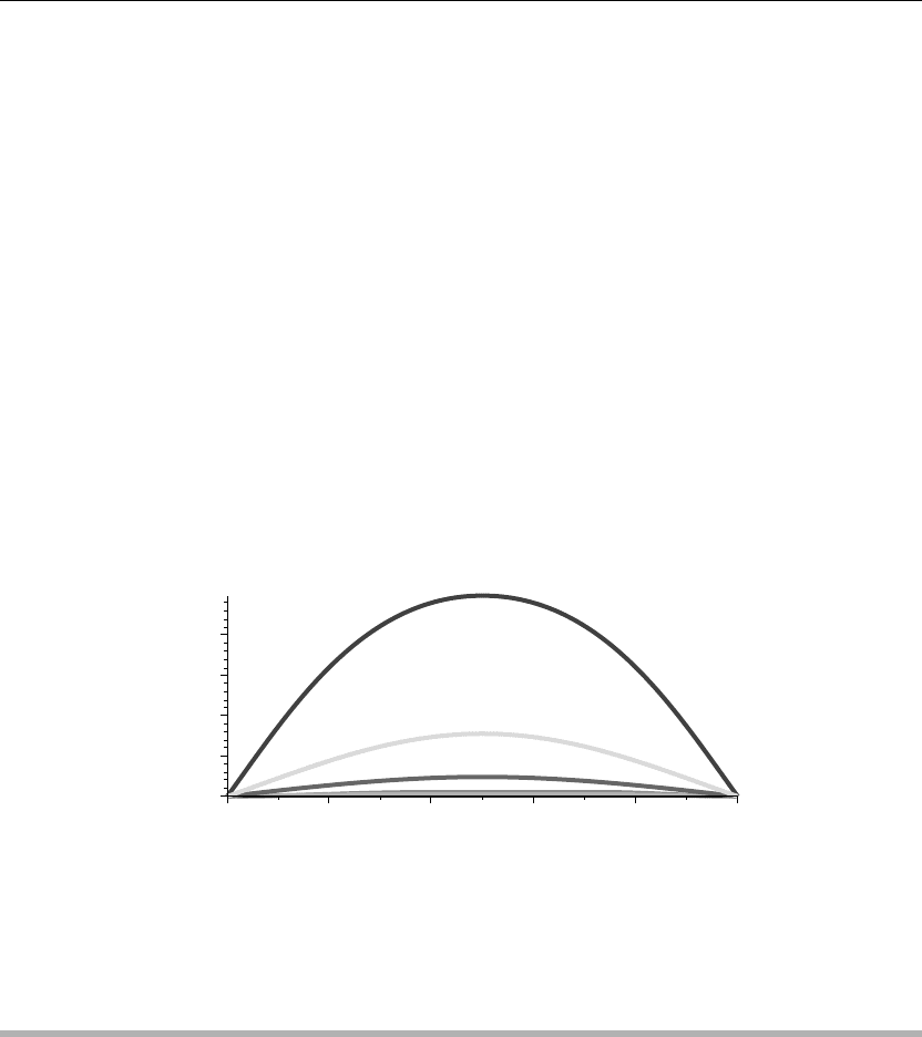
Due to the additional heat loss from the lateral surface, we see that the temperature drops off
more rapidly than in Example 3.6.1.
The preceding animation command illustrates the spatial-time-dependent solution for u(x, t).
The animation sequence shown in Figure 3.6 shows snapshots at times t = 0, 1, 2, 3, 4, and 5.
ANIMATION SEQUENCE
> u(x,0):=subs(t=0,u(x,t)):u(x,1):=subs(t=1,u(x,t)):
> u(x,2):=subs(t=2,u(x,t)):u(x,3):=subs(t=3,u(x,t)):
> u(x,4):=subs(t=4,u(x,t)):u(x,5):=subs(t=5,u(x,t)):
> plot({u(x,0),u(x,1),u(x,2),u(x,3),u(x,4),u(x,5),},x=a..b,thickness=10);
x
0 0.2 0.4 0.6 0.8 1
0
0.05
0.10
0.15
0.20
Figure 3.6
3.7 Verification of Solutions—Three-Step Verification
Procedure
Earlier, we used the method of separation of variables to construct solutions to the initial
value-boundary value problems. The natural question that arises is, does the solution satisfy all
the conditions of the problem? We establish a three-step verification procedure:
1. Does the solution satisfy the partial differential equation?
2. Does the solution satisfy the boundary conditions?
3. Does the solution satisfy the initial conditions?

The Diffusion or Heat Partial Differential Equation 187
To answer all of these questions, we must first deal with some procedural problems that come
about from having to take derivatives of infinite series. For a finite series, such problems do not
exist because from ordinary calculus, we know that the derivative of a sum equals the sum of
the derivatives. However, when the sum is an infinite sum, the preceding may or may not be
true. We now list some theorems, without proof, that will play a role in the verification
procedure for solutions of the preceding problems over the rectangular domain
D ={(x, t) |a<x<b,t>0}.
Theorem 3.7.1 (Convergence of Derivatives) Consider the following infinite series:
u(x) =
∞
n=0
u
n
(x)
If all the series terms u
n
(x) are differentiable on I =[a, b] and if the series of differentiated
terms
∞
n=0
d
dx
u
n
(x)
converges uniformly on I, then the series converges uniformly to the function u(x) and the
derivative of the series equals the series of the derivatives; that is,
d
dx
u(x) =
∞
n=0
d
dx
u
n
(x)
for all x in I.
Theorem 3.7.2 (The Weierstrass M-test for Uniform Convergence) If the terms of the
preceding series satisfy the condition
|
u
n
(x)
|
≤ M
n
for all n and for all x in I =[a, b], where the M
n
are constants (independent of x), and if the
series of constants
∞
n=0
M
n
converges, then the series
∞
n=0
u
n
(x)
converges uniformly for all x in the interval I .
