Ahsan A. (ed.) Evaporation, Condensation and Heat transfer

Подождите немного. Документ загружается.

Two Phase Flow Experimental Study Inside a Microchannel:

Influence of Gravity Level on Local Boiling Heat Transfer

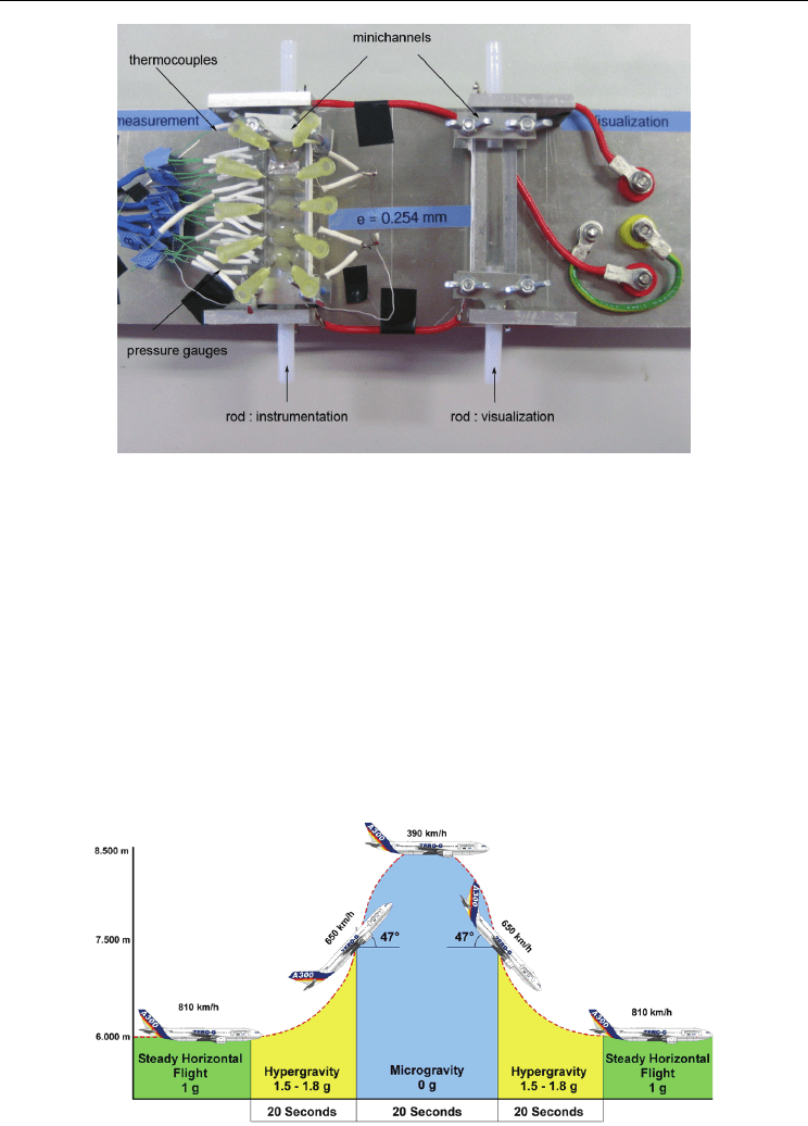
Fig. 5. Coupling of the two minichannels used during parabolic flights (left minichannel for

measurements - right minichannel for visualization).

3.2 Experience in microgravity

3.2.1 On board experiment

The experimental activities are performed in the frame of the MAP (Microgravity

Application Program) Boiling project founded by ESA and embarked on A300-ZeroG to

perform three Parabolic Flights campaigns. The experimental device has been embarked on

board A300 Zero-G to perform three Parabolic Flights campaigns. The Airbus A-300 Zero G

parabolic flight generally executes a series of 31 parabolic manoeuvres during a flight. The

aircraft executes a series of manoeuvre called parabola each providing 20 seconds of

reduced gravity, during which we are able to perform experiments and obtain data that we

are presenting here. During a flight campaign, there are 3 flights with around 31 parabola

begin executed per flight. The period between the start of each parabola is 3 min (Fig. 6):

Fig. 6. The different gravity levels occurring during a parabola.

Evaporation, Condensation and Heat Transfer

Each manoeuvre begins with the aircraft flying in a steady horizontal position, with an

approximate altitude and speed of respectively 6000 m and 810 km.h

-1

. During this steady

flight, the gravity level is 1g. At a set point, the pilot gradually pulls the nose of the aircraft

and it starts climbing. This phase lasts about 20 seconds during which the aircraft

experiences an acceleration between 1,5 and 1,8 g times the gravity level. At an altitude of

7500 meters, with an angle around 47 degrees to the horizontal and with air speed of 650

km.h

-1

, the engine thrust is reduced to the minimum required to compensate.

At this point, the aircraft follows a free-fall ballistic trajectory, i.e. a parabola, lasting

approximately 20 seconds during which the gravity is near zero - the microgravity phase

begins. The peak of the parabola is achieved at around 8500 meters where the speed is about

390 km.h

-1

. At the end of this period when the altitude is 7500 m, the aircraft must pull out

the parabolic arc, a manoeuvre which gives rise to another 20 seconds period of 1,8g, we are

in hypergravity. At the end of the 20 seconds, the aircraft flies a steady horizontal path at 1g

maintaining an altitude of 6000 m.

3.2.2 Microgravity observation

We show the results in microgravity. Concerning the flow behaviour, generally,

microgravity conditions lead to a larger bubble size which is accompanied by deterioration

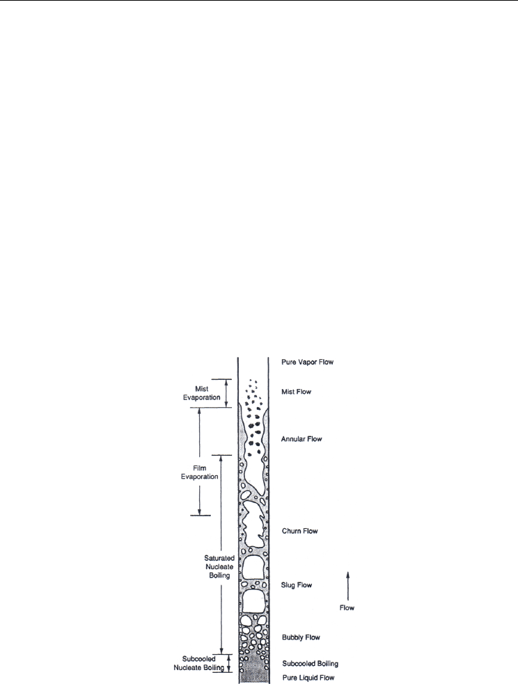
in the heat transfer rate. For low quality, gravity influence is not negligible. On Fig. 7, we

see, for a vertical minichannel, the different flow behaviours during evaporation (Carey,

1992):

Fig. 7. Vertical co-current flow behaviour with evaporation.

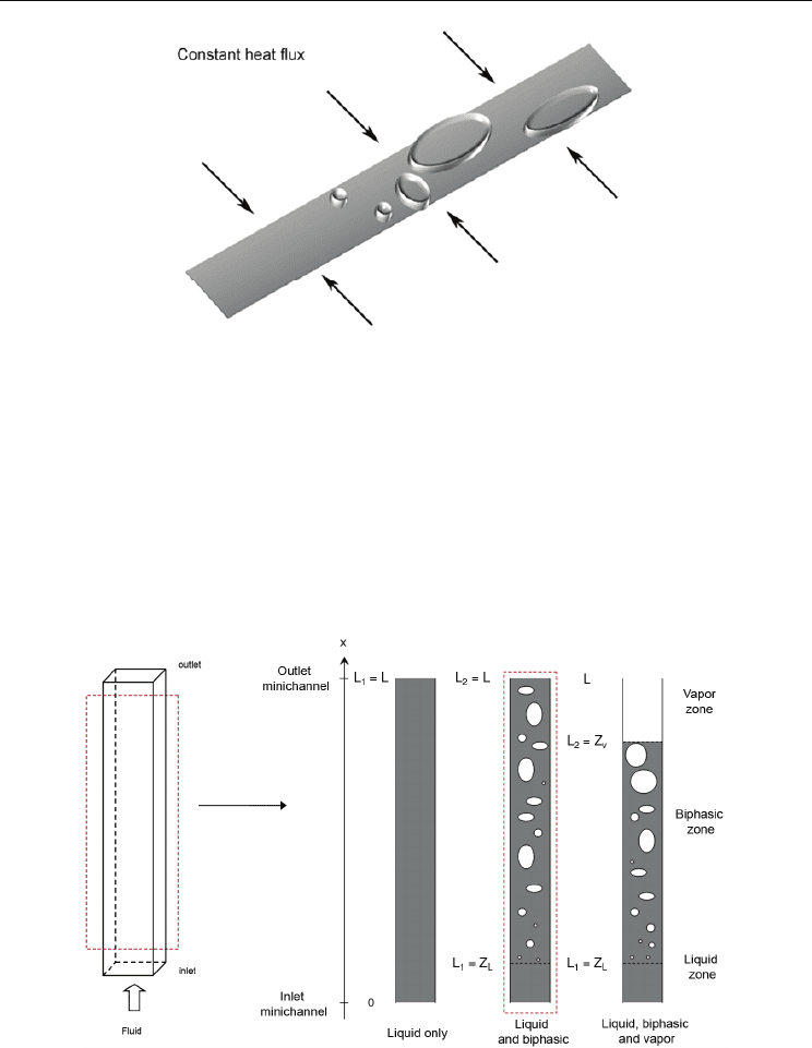
The Fig. 8 shows a typical 3D flow scheme in our minichannel which occurs during a

parabola depending on the heat flux density.

Two Phase Flow Experimental Study Inside a Microchannel:

Influence of Gravity Level on Local Boiling Heat Transfer

Fig. 8. Typical 3D flow scheme occurring in our minichannel.

The differences introduced by gravity level on flow structures are obtained using the data of

parabolic flights (PF63) in March 2007. The analysis (Fig. 9) of the movies recorded

highlights that on the minichannel inlet the flow has a low percentage of insulated bubbles.

The more significant the sizes of the bubbles are, the larger the surface of the super-heated

liquid is. Besides, concerning the microgravity phase, the results present variations

compared to the terrestrial gravity and the hypergravity, which shows an influence of the

gravity level on the confined flow boiling.

To avoid the high wall temperatures and the poor heat transfer associated with the

saturated film boiling regime, the vaporization must be accomplished at low superheat or

low heat flux levels.

Fig. 9. Flow boiling analysis in our minichannel using a fast cam.

The thermal study of the transfers confirms a higher heat transfer coefficient in the input

minichannel during the phase of microgravity (Fig. 13). This decrease is due to the decrease

in size of the vapour bubbles.

Evaporation, Condensation and Heat Transfer

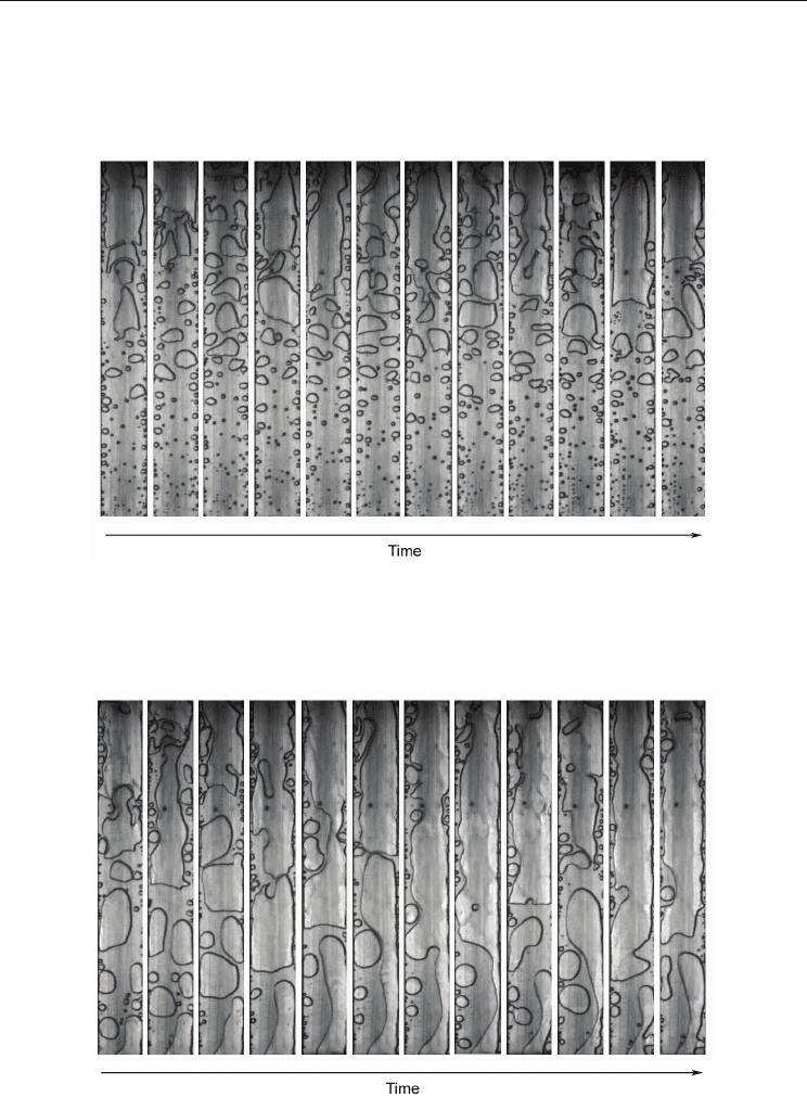
On Fig. 10 and Fig. 11, we plot the evolution of the flow in respectively terrestrial and

microgravity phase during nearly 20 seconds. We can see that there are very big differences

with the structure of the bubbles. In terrestrial gravity, we have bubbly flow profiles while

in microgravity we deal with slug and churn flow according to Fig. 7. Here, we can see the

observations made in terrestrial gravity:

Fig. 10. Flow boiling occurring in our minichannel under terrestrial gravity phase

(20 seconds, Q

=45 kW.m

-2

Then in microgravity, we observed the flow sequence which evidences a different topology

and particularly with the bubble’s size.

Fig. 11. Flow boiling occurring in our minichannel under microgravity phase (20 seconds,

=45 kW.m

-2

Two Phase Flow Experimental Study Inside a Microchannel:

Influence of Gravity Level on Local Boiling Heat Transfer

3.3 Bubble behaviour

To understand fully the role of microgravity on flow boiling and particularly on the bubbles

patterns, we introduce the capillarity length. In fluid mechanics, capillary length is a

characteristic length scale for fluid subject to a body force from gravity and a surface force

due to surface tension. This number function of the

(1)

We can see that the capillarity length depends on g

-0.5.

Or g is the only parameter that

changes during a parabola at a constant mass flow and heat flux rate. Thus when we pass

from 1g to 1.8g, L

decreases of 74 % whereas when we pass from 1g to µg, L

increases of

nearly 1400 %. This may explain the different sizes of the bubbles during microgravity.

Whatever the gravity level, as soon as the vapour occupies the entire minichannel, the heat

transfer coefficient decreases strongly to reach a level which characterizes a kind of vapour

phase heat transfer. Furthermore, as soon as the vapour completely fills the pipe, the heat

exchange strongly falls (Fig. 18). The thermal study of the transfers confirms a higher heat

transfer coefficient in the input minichannel during the phase of microgravity.

3.4 Validation

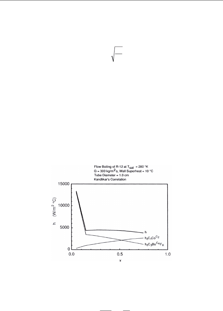
3.4.1 Kandlikar’s correlation

Very recently, (Kandlikar, 2001) proposed a correlation (see below) as a fit to a very broad

spectrum of data for flow boiling heat transfer in vertical and horizontal channels:

Fig. 12. Convective boiling heat transfer coefficient variation with quality level x (here χ

) for

Kandlikar’s correlation.

()

11o le 3 K

h h C C 25Fr C Bo F

⎡

⎤

⎣

⎦

0.8 0.5

−ρ

⎛⎞⎛⎞

⎜⎟

⎝⎠

(2)

Evaporation, Condensation and Heat Transfer

The table below are useful to calculate the Fk number.

Fluid Fk

Water 1.00

R-11 1.30

R-12 1.50

R-13B1 1.31

R-22 2.20

Nitrogen 4.70

Neon 3.50

Fluid Fk

Water 1.00

R-11 1.30

Table 2. List of Fk values for different fluids

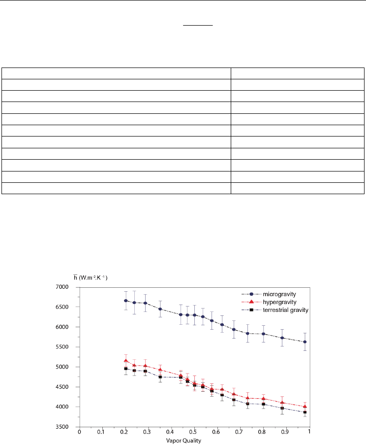
3.4.2 Experimental results

The results are in good agreement with the correlation (Fig. 13). Concerning the range from

0 to 5000 W.m

-2

-1

, we can see that the experimental curves in terrestrial gravity have the

same curvature with the theoretical correlation. Indeed, we have the same level.

Fig. 13. Influence of vapour quality on the heat transfer coefficient in the minichannel

=45 kW.m

-2

3.4.3 Featuring experiments

We can see that we have been able to quantify the heat transfers inside our minichannels

and to validate the experimental results in normal gravity with correlation found in

literature. So for terrestrial conditions, the results are validated.

Two Phase Flow Experimental Study Inside a Microchannel:

Influence of Gravity Level on Local Boiling Heat Transfer

Now, we are going to present more results concerning the influence of three parameters on

the heat transfers: the gravity level, the Reynolds number and the Vapour quality. We are

presenting and analysing experimental results.

4. Heat transfer results

4.1 Inverse method

Here, we introduce quickly the estimation method to explain how we estimate our

parameter (Le Niliot, 2001). It consists in inversing experimental data measurements

(thermocouples) to obtain the surface temperature and the surface flux density in the

minichannel. The inverse problem deals with the resolution of IHCP (Beck et al, 1985) where

we want to estimate the unknown boundary conditions on the surface minichannel. The

numerical method used here is the BEM (Brebbia et al, 1984). This method has been applied

in our laboratory for several years to solve inverse problems (Le Niliot et Lefèvre, 2001).

BEM is attractive for our inverse problem resolution because it provides a direct connection

between the unknown boundary heat flux, the measurements (thermocouples here) and the

linear heat sources (heating wires here). The solution can be obtained by solving a linear

system of simultaneous equations without any iterative process.

The estimation procedure consists in inversing the temperature measurements under the

minichannel in order to estimate the local boiling heat transfer coefficient h(x), knowing the

local heat flux and the local surface temperatures (

surface

T ). Those functions of

space are the results of the inverse problem. The estimation of the solution is obtained as the

solution of the following optimization problem:

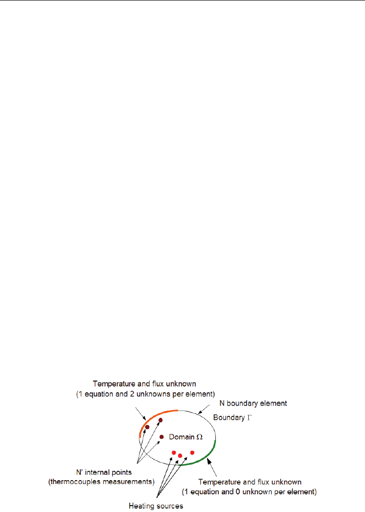
4.1.1 Boundary estimation

As N' is the number of domain Ω interior points given here by the thermocouples and N the

number of boundary elements on our rod, the system has got (N+N') equations. The number

of unknowns, noted M, is a function of the boundary conditions applied on the different

elements of Γ ( Fig. 14). Namely for element Γ

we have at least one unknown per element

for the following boundary conditions:

First kind condition for which heat flux ϕi is unknown and temperature θ

is imposed.

Second kind condition for which temperature θi unknown and heat flux ϕ

is imposed.

Third kind condition ϕi=f(θi)

Fig. 14. The problem of the unknown boundary conditions.

Evaporation, Condensation and Heat Transfer

The elements, for which we have one equation, where the boundary condition is missing, let

appear two unknowns. The only way to solve the fundamental heat transfer equation is to

find some extra information, provided by measurements. In our case, we have interior

measurements, given by thermocouples. They enable us with the knowledge of the

boundary conditions to solve the problem and to calculate local heat flux and local surface

temperatures along the minichannel. This estimation procedure consists in inversing the

temperature measurements under the minichannel in order to estimate the local boiling heat

transfer coefficient h(x). Those functions of space are the results of the inverse problem. The

estimation of the solution is obtained using BEM as the solution of the following

optimization problem:

()

{

}

mod meas

ˆˆ

surface surface

−φ =arg min (3)

In this last expression, the vectors

meas

T and

mod

T respectively represent the vector of

temperature measurements and the vector of the calculated temperatures. The unknown

factors (

surface

) are obtained by minimizing the difference between measurements

and a mathematical modeling. Taking into account the specificity of formulation BEM

., this

minimization is not obtained explicitly but done through a function utilizing a linear

combination of measurements. This formulation leads to a matrix system of simultaneous

equation :

X=BA

(4)

In this last equation,

A is a matrix of dimension ((N+N)'×M), X the vector of the M

unknowns including (

surface

) and B of dimension (N+N') is containing a linear

combination of the data measurements. If M=N+N' we obtain a square system of linear

equation but most of the time we have M<N+N' and has more equations than unknown (see

Sensitivity Study chapter) : our system presents 270 equations for 255 unknown factors

(overdetermined system). A solution can be found by minimising the distance between

vector

AX and vector B. In order to find out an estimation

of the unknown exact solution

X, we have to solve the optimization problem using a cost function (5). Assuming that the

difference between

AX and B can be considered as distributed according a Gaussian law we

can find

solution of in the meaning of the least squares. Using this last property leads to

the Ordinary Least Squares solution :

⎧

⎫

⎛⎞

⎜⎟

⎨

⎬

⎝⎠

⎩⎭

X=arg min AX-B

(5)

()()

X= B

AA A (6)

Actually, the inverse heat condition problem is ill-posed and very sensitive to the

measurements errors. Considering the numerical aspects of the inversion, we obtain an ill-

conditioned square matrix (

A). Thus, we observe for the system numerical resolution an

instability of the solution

with regards to the measurements the errors introduced into

the vector

B. As a consequence, we need to obtain a stable the solution of this system by

using regularizations tools – Hansen. We propose in the following paragraph an example of

Two Phase Flow Experimental Study Inside a Microchannel:

Influence of Gravity Level on Local Boiling Heat Transfer

regularization procedure which can be applied. In order to smooth the solution, we used in

our our study the Lanczos decomposition called the the SVD method.

4.1.2 Regularization using SVD

The regularization of an inverse problem consists in adding information to improve the

stability of the solution with regards to the measurements noise and/or to select a type of

solution among all those possible. The ill-conditioned character of matrix

A results in the

presence of low singular values. They are a consequence of linear dependent equations :

indication of a strong correlation between the unknown factors.

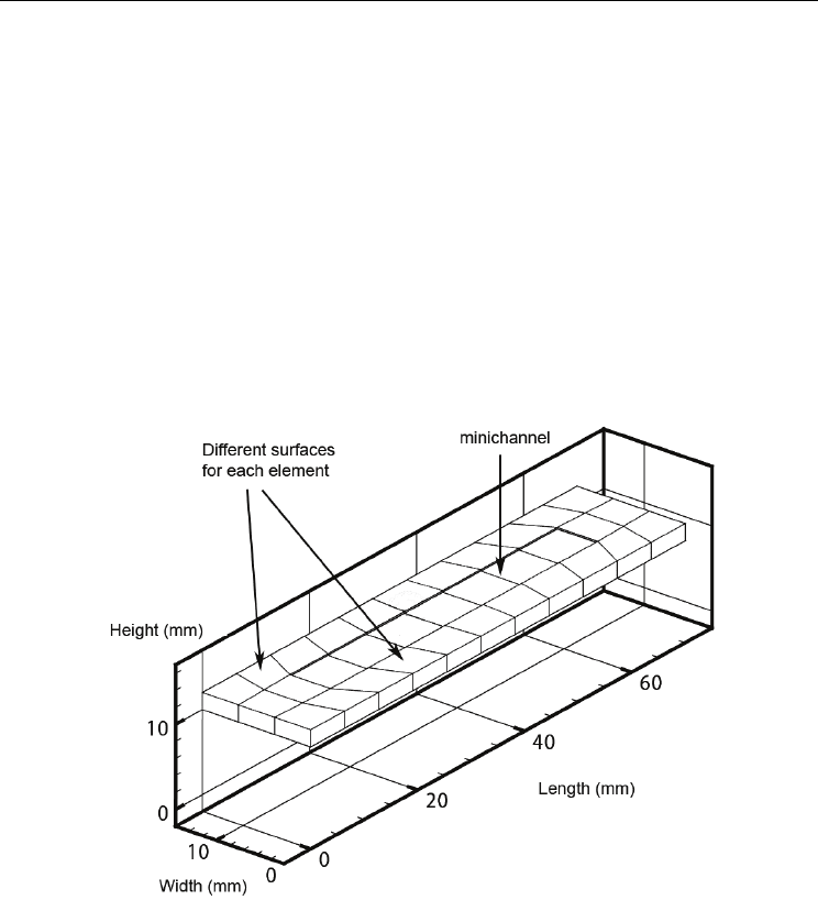
Actually, the SVD method makes possible to deal with 3D inverse problem where the mesh

is structured, i.e. the pavements of the elements do not have all the same surfaces and thus

the same sensitivity (Fig. 15). This property increased the ill-poseness of the problem.

Indeed, the solution is much more unstable when the space discretization is refined. This

singular behavior is due to the fact that the conditioning number of the linear system (see

the L-curve paragraph) is a function of the power of the meshing step.

Fig. 15. 3D Meshing- of the minichannel only the faces are meshed.

In our problem, SVD method consists in removing the too small singular values which affect

the stability of the system in order to find one solution among several, which best

corresponds. It can seem contradictory to improve the system by removing equations and

thus information : the suppression of the equations involves a reduction in the rank of our

system and consequently an increase in the space of the plausible solutions. However, the

action of removing these equations improves the stability because it deliberately removes

the equations which disturb the solution. Matrix

A can be built into a product of squares

matrices (

U and V are orthogonal matrices and W is the diagonal matrix of the singular

values

) as shown :

Evaporation, Condensation and Heat Transfer

AUWV=

XUDia

⎛⎞

⎜⎟

⎝⎠

(7)

A is ill-conditioned when some singular values w

→ 0 (1/w

→ ∞ ).As a result, the errors are

increased. By using SVD, W

-1

is truncated from the too high (1/w

⎡

⎤

⎢

⎥

⎢

⎥

⎢

⎥

⎢

⎥

⎢

⎥

⎢

⎥

⎣

⎦

#% #

#%#

"""

(8)

The truncated matrix can be built up as in:

⎡

⎤

⎢

⎥

⎢

⎥

⎢

⎥

⎢

⎥

⎢

⎥

⎢

⎥

⎣

⎦

#% #

#%#

(9)

The estimate solution vector

is function of the new truncated matrix

−

(

)

XUWVB

−

(10)

We observe like in the regularization method by modifications of the functions to be

minimised (for example Tikhonov) a smoothing of the solution. However, it is necessary to

explain how is carried out the choice of the singular values ignored. There is a “criteria”

making it possible to quantify the balance between a stable solution and low residuals : the

condition number. It is defined by the ratio of the highest to the weakest of the singular

values of matrix A.

All the singular values lower than a limit value are eliminated. The numerical procedure can

be found in the LINPACK or in Numerical recipes (Press et al, 1990). This technique requires

the use of a threshold which allows the choice of values to be cancelled. The level of

truncation is determined by the technique known as the L-curve (Hansen, 1998).

4.1.3 The L-curve

The obtained solution

depends on a value selected by the user. To avoid entering

extremes and losing information, a tool called L-curve is introduced to estimate the correct

condition number. The goal is to trace on a logarithmic scale the norm of the solution on the

norm of the residuals

AX-B

(Fig. 16).

The optimal value is in the hollow of the L where the best compromise between stable

results and low residuals (on the distinct corner separating the vertical and the horizontal

part of the curve). It is around this corner that we find the best compromise.