A Modern Introduction to Probability and Statistics, Understanding Why and How - Dekking, Kraaikamp, Lopuhaa, Meester (Современное введение в теорию вероятностей и статистику - Как? и Почему? )
Подождите немного. Документ загружается.


A
Summary of distributions
Discrete distributions
1. Bernoulli distribution: Ber (p), where 0 ≤ p ≤ 1.
P(X =1)=p and P(X =0)=1− p.
E[X]=p and Var(X)=p(1 − p).
2. Binomial distribution: Bin(n, p), where 0 ≤ p ≤ 1.
P(X = k)=
n
k
p
k
(1 − p)
n−k
for k =0, 1,...,n.
E[X]=np and Var(X)=np(1 − p).
3. Geometric distribution: Geo(p), where 0 <p≤ 1.
P(X = k)=p(1 − p)
k−1
for k =1, 2,... .
E[X]=1/p and Var(X)=(1− p)/p
2
.
4. Poisson distribution: Pois(µ), where µ>0.
P(X = k)=
µ
k
k!
e
−µ
for k =0, 1,... .
E[X]=µ and Var(X)=µ.
Continuous distributions
1. Cauchy distribution: Cau(α, β), where −∞ <α<∞ and β>0.
f(x)=
β
π (β
2
+(x − α)
2
)
for −∞ <x<∞.
F (x)=
1
2
+
1
π
arctan
x − α
β
for −∞ <x<∞.
E[X]andVar(X)donotexist.

430 A Summary of distributions
2. Exponential distribution: Exp(λ), where λ>0.
f(x)=λe
−λx
for x ≥ 0.
F (x)=1− e
−λx
for x ≥ 0.
E[X]=1/λ and Var(X)=1/λ
2
.
3. Gamma distribution: Gam(α, λ), where α>0andλ>0.
f(x)=
λ (λx)
α−1
e
−λx
Γ(α)
for x ≥ 0.
F (x)=
x
0
λ (λt)
α−1
e
−λt
Γ(α)
dt for x ≥ 0.
E[X]=α/λ and Var(X)=α/λ
2
.
4. Normal distribution: N(µ, σ
2
), where −∞ <µ<∞ and σ>0.
f(x)=
1
σ
√
2π
e
−
1
2
x−µ
σ
2
for −∞ <x<∞.
F (x)=
x
−∞
1
σ
√
2π
e
−
1
2
t−µ
σ
2
dt for −∞ <x<∞.
E[X]=µ and Var(X)=σ
2
.
5. Pareto distribution: Par(α), where α>0.
f(x)=
α
x
α+1
for x ≥ 1.
F (x)=1− x
−α
for x ≥ 1.
E[X]=α/(α − 1) for α>1and∞ for 0 <α≤ 1.
Var(X)=α/((α − 1)
2
(α − 2)) for α>2and∞ for 0 <α≤ 1.
6. Uniform distribution: U(a, b), where a<b.
f(x)=
1
b − a
for a ≤ x ≤ b.
F (x)=
x − a
b − a
for a ≤ x ≤ b.
E[X]=(a + b)/2andVar(X)=(b − a)
2
/12.

B
Tables of the normal and t-distributions

432 B Tables of the normal and t-distributions
Table B.1. Right tail probabilities 1 − Φ(a)=P(Z ≥ a) for an N (0, 1) distributed
random variable Z.
a 0123456789
0.0 5000 4960 4920 4880 4840 4801 4761 4721 4681 4641
0.1 4602 4562 4522 4483 4443 4404 4364 4325 4286 4247
0.2 4207 4168 4129 4090 4052 4013 3974 3936 3897 3859
0.3 3821 3783 3745 3707 3669 3632 3594 3557 3520 3483
0.4 3446 3409 3372 3336 3300 3264 3228 3192 3156 3121
0.5 3085 3050 3015 2981 2946 2912 2877 2843 2810 2776
0.6 2743 2709 2676 2643 2611 2578 2546 2514 2483 2451
0.7 2420 2389 2358 2327 2296 2266 2236 2206 2177 2148
0.8 2119 2090 2061 2033 2005 1977 1949 1922 1894 1867
0.9 1841 1814 1788 1762 1736 1711 1685 1660 1635 1611
1.0 1587 1562 1539 1515 1492 1469 1446 1423 1401 1379
1.1 1357 1335 1314 1292 1271 1251 1230 1210 1190 1170
1.2 1151 1131 1112 1093 1075 1056 1038 1020 1003 0985
1.3 0968 0951 0934 0918 0901 0885 0869 0853 0838 0823
1.4 0808 0793 0778 0764 0749 0735 0721 0708 0694 0681
1.5 0668 0655 0643 0630 0618 0606 0594 0582 0571 0559
1.6 0548 0537 0526 0516 0505 0495 0485 0475 0465 0455
1.7 0446 0436 0427 0418 0409 0401 0392 0384 0375 0367
1.8 0359 0351 0344 0336 0329 0322 0314 0307 0301 0294
1.9 0287 0281 0274 0268 0262 0256 0250 0244 0239 0233
2.0 0228 0222 0217 0212 0207 0202 0197 0192 0188 0183
2.1 0179 0174 0170 0166 0162 0158 0154 0150 0146 0143
2.2 0139 0136 0132 0129 0125 0122 0119 0116 0113 0110
2.3 0107 0104 0102 0099 0096 0094 0091 0089 0087 0084
2.4 0082 0080 0078 0075 0073 0071 0069 0068 0066 0064
2.5 0062 0060 0059 0057 0055 0054 0052 0051 0049 0048
2.6 0047 0045 0044 0043 0041 0040 0039 0038 0037 0036
2.7 0035 0034 0033 0032 0031 0030 0029 0028 0027 0026
2.8 0026 0025 0024 0023 0023 0022 0021 0021 0020 0019
2.9 0019 0018 0018 0017 0016 0016 0015 0015 0014 0014
3.0 0013 0013 0013 0012 0012 0011 0011 0011 0010 0010
3.1 0010 0009 0009 0009 0008 0008 0008 0008 0007 0007
3.2 0007 0007 0006 0006 0006 0006 0006 0005 0005 0005
3.3 0005 0005 0005 0004 0004 0004 0004 0004 0004 0003
3.4 0003 0003 0003 0003 0003 0003 0003 0003 0003 0002

B Tables of the normal and t-distributions 433
Table B.2. Right critical values t
m,p
of the t-distribution with m degrees of freedom
corresponding to right tail probability p:P(T
m
≥ t
m,p
)=p. The last row in the table
contains right critical values of the N (0, 1) distribution: t
∞,p
= z
p
.
Right tail probability p
m 0.1 0.05 0.025 0.01 0.005 0.0025 0.001 0.0005
1 3.078 6.314 12.706 31.821 63.657 127.321 318.309 636.619
2 1.886 2.920 4.303 6.965 9.925 14.089 22.327 31.599
3 1.638 2.353 3.182 4.541 5.841 7.453 10.215 12.924
4 1.533 2.132 2.776 3.747 4.604 5.598 7.173 8.610
5 1.476 2.015 2.571 3.365 4.032 4.773 5.893 6.869
6 1.440 1.943 2.447 3.143 3.707 4.317 5.208 5.959
7 1.415 1.895 2.365 2.998 3.499 4.029 4.785 5.408
8 1.397 1.860 2.306 2.896 3.355 3.833 4.501 5.041
9 1.383 1.833 2.262 2.821 3.250 3.690 4.297 4.781
10 1.372 1.812 2.228 2.764 3.169 3.581 4.144 4.587
11 1.363 1.796 2.201 2.718 3.106 3.497 4.025 4.437
12 1.356 1.782 2.179 2.681 3.055 3.428 3.930 4.318
13 1.350 1.771 2.160 2.650 3.012 3.372 3.852 4.221
14 1.345 1.761 2.145 2.624 2.977 3.326 3.787 4.140
15 1.341 1.753 2.131 2.602 2.947 3.286 3.733 4.073
16 1.337 1.746 2.120 2.583 2.921 3.252 3.686 4.015
17 1.333 1.740 2.110 2.567 2.898 3.222 3.646 3.965
18 1.330 1.734 2.101 2.552 2.878 3.197 3.610 3.922
19 1.328 1.729 2.093 2.539 2.861 3.174 3.579 3.883
20 1.325 1.725 2.086 2.528 2.845 3.153 3.552 3.850
21 1.323 1.721 2.080 2.518 2.831 3.135 3.527 3.819
22 1.321 1.717 2.074 2.508 2.819 3.119 3.505 3.792
23 1.319 1.714 2.069 2.500 2.807 3.104 3.485 3.768
24 1.318 1.711 2.064 2.492 2.797 3.091 3.467 3.745
25 1.316 1.708 2.060 2.485 2.787 3.078 3.450 3.725
26 1.315 1.706 2.056 2.479 2.779 3.067 3.435 3.707
27 1.314 1.703 2.052 2.473 2.771 3.057 3.421 3.690
28 1.313 1.701 2.048 2.467 2.763 3.047 3.408 3.674
29 1.311 1.699 2.045 2.462 2.756 3.038 3.396 3.659
30 1.310 1.697 2.042 2.457 2.750 3.030 3.385 3.646
40 1.303 1.684 2.021 2.423 2.704 2.971 3.307 3.551
50 1.299 1.676 2.009 2.403 2.678 2.937 3.261 3.496
∞ 1.282 1.645 1.960 2.326 2.576 2.807 3.090 3.291

C
Answers to selected exercises
2.1 P(A ∪ B)=13/18.
2.4 Yes.
2.7 0.7.
2.8 P(D
1
∪ D
2
) ≤ 2 · 10
−6
and
P(D
1
∩ D
2
) ≤ 10
−6
.
2.11 p =(−1+
√
5)/2.
2.12 a 1/10!
2.12 b 5! · 5!
2.12 c 8/63 = 12.7percent.
2.14 a
ab c
a 01/61/6
b 001/3
c 01/30
2.14 b P({(a, b), (a, c)})=1/3.
2.14 c P({(b, c), (c, b)})=2/3.
2.16 P(E)=2/3.
2.19 a Ω={2, 3, 4,...}.
2.19 b 4p
2
(1 − p)
3
.
3.1 7/36.
3.2 a P(A |B)=2/11.
3.2 b No.
3.3 a P(S
1
)=13/52 = 1/4,
P(S
2
|S
1
)=12/51, and
P(S
2
|S
c
1
)=13/51.
3.3 b P(S
2
)=1/4.
3.4 P(B |T )=9.1 · 10
−5
and
P(B |T
c
)=4.3 · 10
−6
.
3.7 a P(A ∪ B)=1/2.
3.7 b P(B)=1/3.
3.8 a P(W )=0.117.
3.8 b P(F |W )=0.846.
3.9 P(B |A)=7/15.
3.14 a P(W |R)=0andP(W |R
c
)=1.
3.14 b P(W )=2/3.
3.16 a P(D |T )=0.165.
3.16 b 0.795.
4.1 a a 012
p
Z
(a)25/36 10/36 1/36
Z has a Bin(2, 1/6) distribution.
4.1 b {M =2,Z =0} = {(2, 1), (1, 2),
(2, 2) }, {S =5,Z =1} = ∅,and
{S =8,Z =1} = {(6, 2), (2, 6) }.
P(M =2,Z =0)=1/12,
P(S =5,Z = 1) = 0, and
P(S =8,Z =1)=1/18.
4.1 c The events are dependent.
4.3 a 01/23/4
p(a)1/31/61/2
4.6 a p
¯
X
(1) = p
¯
X
(3) = 1/27, p
¯
X
(4/3) =
p
¯
X
(8/3) = 3/27, p
¯
X
(5/3) = p
¯
X
(7/3) =
6/27, and p
¯
X
(2) = 7/27.
4.6 b 6/27.

436 C Answers to selected exercises
4.7 a Bin(1000, 0.001).
4.7 b P(X =0) = 0.3677, P(X =1) =
0.3681, and P(X>2) = 0.0802.
4.8 a Bin(6, 0.8178).
4.8 b 0.9999634.
4.10 a Determine P(R
i
=0)first.
4.10 b No!
4.10 c See the birthday problem in Sec-
tion 3.2.
4.12 No!
4.13 a Geo(1/N ).
4.13 b Let D
i
be the event that the
marked bolt was drawn (for the first
time) in the ith draw, and use condi-
tional probabilities in
P(Y = k)=P(D
c
1
∩···∩D
c
k−1
∩ D
k
).
4.13 c Count the number of ways the
event {Z = k} can occur, and divide this
by the number of ways
N
r
we can select
r objects from N objects.
5.2 P(1/2 <X≤ 3/4) = 5/16.
5.4 a P(X<41/2) = 1/4.
5.4 b P(X = 5)=1/2.
5.4 c X is neither discrete nor continu-
ous!
5.5 a c =1.
5.5 b F (x)=0forx ≤−3;
F (x)=(x +3)
2
/2for−3 ≤ x ≤−2;
F (x)=1/2for−2 ≤ x ≤ 2;
F (x)=1− (3 − x)
2
/2for2≤ x ≤ 3;
F (x)=1forx ≥ 3.
5.8 a g(y)=1/(2
√
ry).
5.8 b Yes.
5.8 c Consider F (r/10).
5.9 a 1/2 and {(x, y):2≤x ≤ 3, 1 ≤ y ≤
3/2}.
5.9 b F (x)=0forx<0;
F (x)=2x for 0 ≤ x ≤ 1/2;
F (x)=1forx>1/2.
5.9 c f(x)=2for0≤ x ≤ 1/2;
f(x)=0elsewhere.
5.12 2.
5.13 a Change variables from x to −x.
5.13 b P(Z ≤−2) = 0.0228.
6.2 a 1+2
√
0.378 ··· =2.2300795.
6.2 b Smaller.
6.2 c 0.3782739.
6.5 Show, for a ≥ 0, that X ≤ a is
equivalent with U ≥ e
−a
.
6.6 U =e
−2X
.
6.7 Z =
−ln(1 − U)/5, or
Z =
−ln U/5.
6.9 a 6/8.
6.9 b Geo(6/8).
6.10 a Define B
i
=1ifU
i
≤ p and
B
i
=0ifU
i
>p,andN as the posi-
tion in the sequence of B
i
where the first
1 occurs.
6.10 b P(Z>n)=(1− p)
n
,forn =
0, 1,...; Z has a Geo (p) distribution.
7.1 a Outcomes:1,2,3,4,5,and6.Each
has probability 1/6.
7.1 b E[T ]=7/2, Var(T )=35/12.
7.2 a E[X]=1/5.
7.2 b y 01
P(Y = y)2/53/5
and E [Y ]=3/5.
7.2 c E
X
2
=3/5.
7.2 d Var(X)=14/25.
7.5 E[X]=p and Var(X)=p(1 − p).
7.6 195/76.
7.8 E[X]=1/3.
7.10 a E[X]=1/λ and E
X
2
=2/λ
2
.
7.10 b Var(X)=1/λ
2
.
7.11 a 2.
7.11 b The expectation is infinite!
7.11 c E[X]=
∞
1
x · αx
−α−1
dx.
7.15 a Start with
Var(rX)=E
(rX − E[rX])
2
.
7.15 b Start with Var(X + s)=
E
((X + s) − E[X + s])
2
.
7.15 c Apply b with rX instead of X.
7.16 E[X]=4/9.

C Answers to selected exercises 437
7.17 a If positive terms add to zero,
they must all be zero.
7.17 b Note that
E
(V − E[V ])
2
=Var(V ).
8.1 y 01020
P(Y = y) 0.2 0.4 0.4
8.2 a y −10 1
P(Y = y) 1/6 1/2 1/3
8.2 b z −10 1
P(Z = z) 1/3 1/2 1/6
8.2 c P(W =1)=1.
8.3 a V has a U(7, 9) distribution.
8.3 b rU + s has a U (s, s + r) distribu-
tion if r>0andaU (s+r, s) distribution
if r<0.
8.5 a x
2
(3 − x)/4for0≤ x ≤ 2.
8.5 b F
Y
(y)=(3/4)y
4
−(1/4)y
6
for 0 ≤
y ≤
√
2.
8.5 c 3y
3
− (3/2)y
5
for 0 ≤ y ≤
√
2,
0elsewhere.
8.8 F
W
(w)=1− e
−γw
α
,withγ = λ
α
.
8.10 0.1587.
8.11 Apply Jensen with −g.
8.12 a y 0 1 10 100
P(Y = y)
1
4
1
4
1
4
1
4
8.12 b
E[X] ≥ E
√
X
.
8.12 c
E[X]=50.25, but E
√
X
=
27.75.
8.18 V has an exponential distribution
with parameter nλ.
8.19 a The upper right quarter of the
circle.
8.19 b F
Z
(t)=1/2 + arctan(t)/π.
8.19 c 1/[π(1 + z
2
)].
9.2 a P(X =0,Y = −1) = 1/6,
P(X =0,Y =1)=0,
P(X =1,Y = −1) = 1/6,
P(X =2,Y = −1) = 1/6,
and P(X =2,Y =1)=0.
9.2 b Dependent.
9.5 a 1/16 ≤ η ≤ 1/4.
9.5 b No.
9.6 a
u
v 012
0 1/4 0 1/4 1/2
1 0 1/2 0 1/2
1/4 1/2 1/4 1
9.6 b Dependent.
9.8 a z 0123
p
Z
(z)
1
4
1
4
1
4
1
4
9.8 b z −2 −10123
p
˜
X
(z)
1
8
1
8
1
4
1
4
1
8
1
8
9.9 a F
X
(x)=1− e
−2x
for x>0and
F
Y
(y)=1−e
−y
for y>0.
9.9 b f(x, y)=2e
−(2x+y)
for x>0and
y>0.
9.9 c f
X
(x)=2e
−2x
x>0andf
Y
(y)=
e
−y
for y>0.
9.9 d Independent.
9.10 a 41/720.
9.10 b F (a, b)=
3
5
a
2
b
2
+
2
5
a
2
b
3
.
9.10 c F
X
(a)=a
2
.
9.10 d f
X
(x)=2x for 0 ≤ x ≤ 1.
9.10 e Independent.
9.11 27/50.
9.13 a 1/π.
9.13 b F
R
(r)=r
2
for 0 ≤ r ≤ 1.
9.13 c f
X
(x)=
2
π
√
1 − x
2
= f
Y
(x)for
x between −1and1.
9.15 a Since F(a, b)=
area (∆∩(a,b))
area of ∆
,
where (a, b)isthesetofpoints(x, y),
for which x ≤ a and y ≤ b, one needs to
calculate the areas for the various cases.
9.15 b f(x, y)=2for(x, y) ∈ ∆, and
f(x, y)=0otherwise.
9.15 c Use the rule on page 122.
9.19 a a =5
√
2, b =4
√
2, and c = 18.

438 C Answers to selected exercises
9.19 b Use that
1
σ
√
2π
e
−
1
2
y−µ
σ
2
is
the probability density function of an
N(µ, σ
2
) distributed random variable.
9.19 c N (0, 1/36).
10.1 a Cov(X, Y )=0.142. Positively
correlated.
10.1 b ρ (X, Y )=0.0503.
10.2 a E[XY ]=0.
10.2 b Cov(X, Y )=0.
10.2 c Var(X + Y )=4/3.
10.2 d Var(X − Y )=4/3.
10.5 a
a
b 012
0 8/72 6/72 10/72 1/3
1 12/72 9/72 15/72 1/2
2 4/72 3/72 5/72 1/6
1/3 1/4 5/12 1
10.5 b E[X]=13/12, E [Y ]=5/6, and
Cov(X, Y )=0.
10.5 c Yes.
10.6 a E[X]=E[Y ]=0and
Cov(X, Y )=0.
10.6 b E[X]=E[Y ]=c;E[XY ]=c
2
.
10.6 c No.
10.7 a Cov(X, Y )=−1/8.
10.7 b ρ(X, Y )=−1/2.
10.7 c For ε equal to 1/4, 0 or −1/4.
10.9 a P(X
i
=1)=(1−0.001)
40
=0.96
and P(X
i
= 41) = 0.04.
10.9 b E[X
i
]=2.6and
E[X
1
+ ···+ X
25
] = 65.
10.10 a E[X] = 109/50,
E[Y ] = 157/100, and E [X + Y ]=15/4.
10.10 b E
X
2
= 1287/250,
E
Y
2
= 318/125, and
E[X + Y ] = 3633/250.
10.10 c Var(X) = 989/2500,
Var(Y ) = 791/10 000, and
Var(X + Y ) = 4747/10 000.
10.14 a Use the alternative expression
for the covariance.
10.14 b Use the alternative expression
for the covariance.
10.14 c Combine parts a and b.
10.16 a Var(X)+Cov(X, Y ).
10.16 b Anything can happen.
10.16 c X and X +Y are positively cor-
related.
10.18 Solve 0 = N(N −1)(N +1)/12 +
N(N − 1)Cov(X
1
,X
2
).
11.1 a Check that for k between 2 and 6,
the summation runs over =1,...,k−1,
whereas for k between 7 and 12 it runs
over = k − 6,...,12.
11.1 b Check that for 2 ≤ k ≤ N,the
summation runs over =1,...,k − 1,
whereas for k between N +1 and 2N it
runs over = k − N,...,2N.
11.2 a Check that the summation runs
over =0, 1,...,k.
11.2 b Use that λ
k−
µ
/(λ+µ)
k
is equal
to p
1 − p
k−
,withp = µ/(λ + µ).
11.4 a E[Z]=−3andVar(Z) = 81.
11.4 b Z has an N(−3, 81) distribution.
11.4 c P(Z ≤ 6) = 0.8413.
11.5 Check that for 0 ≤ z<1, the in-
tegral runs over 0 ≤ y ≤ z,whereasfor
1 ≤ z ≤ 2, it runs over z − 1 ≤ y ≤ 1.
11.6 Check that the integral runs over
0 ≤ y ≤ z.
11.7 Recall that a Gam (k, λ) random
variable can be represented as the sum of
k independent Exp (λ) random variables.
11.9 a f
Z
(z)=
3
2
1
z
2
−
1
z
4
,forz ≥ 1.
11.9 b f
Z
(z)=
αβ
β − α
1
z
β+1
−
1
z
α+1
,
for z ≥ 1.
12.1 e 1: no, 2: no, 3: okay, 4: okay, 5:
okay.
12.5 a 0.00049.
C Answers to selected exercises 439
12.5 b 1 (correct to 8281 decimals).
12.6 0.256.
12.7 a λ ≈ 0.192.
12.7 b 0.1583 is close to 0.147.
12.7 c 2.71 · 10
−5
.
12.8 a E[X(X − 1)] = µ
2
.
12.8 b Var(X)=µ.
12.11 The probability of the event in
the hint equals (λs)
n
e
−λ2s
/(k!(n − k)!).
12.14 a Note: 1−1/n → 1and1/n → 0.
12.14 b E[X
n
]=(1− 1/n) · 0+(1/n) ·
7n =7.
13.2 a E[X
i
]=0andVar(X
i
)=1/12.
13.2 b 1/12.
13.4 a n ≥ 63.
13.4 b n ≥ 250.
13.4 c n ≥ 125.
13.4 d n ≥ 240.
13.6 Expected income per game
1/37;
per year:
9865.
13.8 a Var
¯
Y
n
/2h
=0.171/h
√
n.
13.8 b n ≥ 801.
13.9 a T
n
is the average of a sequence of
independent and identically distributed
random variables.
13.9 b a =E
X
2
i
=1/3.
13.10 a P(|M
n
− 1| >ε)=(1− ε)
n
for
0 ≤ ε ≤ 1.
13.10 b No.
14.2 0.9977.
14.3 17.
14.4 1/2.
14.5 Use that X has the same probabil-
ity distribution as X
1
+ X
2
+ ···+ X
n
,
where X
1
,X
2
,...,X
n
are independent
Ber(p) distributed random variables.
14.6 a P(X ≤ 25) ≈ 0.5, P(X<26) ≈
0.6141.
14.6 b P(X ≤ 2) ≈ 0.
14.9 a 5.71%.
14.9 b Yes!
14.10 a 91.
14.10 b Use that (
¯
M
n
− c)/σ has an
N(0, 1) distribution.
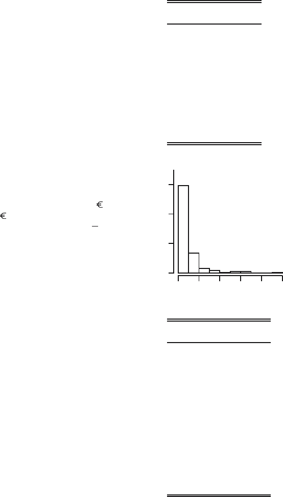
15.3 a
Bin Height
(0,250] 0.00297
(250,500] 0.00067
(500,750] 0.00015
(750,1000] 0.00008
(1000,1250] 0.00002
(1250,1500] 0.00004
(1500,1750] 0.00004
(1750,2000] 0
(2250,2500] 0
(2250,2500] 0.00002
15.3 b Skewed.
0 500 1000 1500 2000 2500
0
0.001
0.002
0.003
15.4 a
Bin Height
[0,500] 0.0012741
(500,1000] 0.0003556
(1000,1500] 0.0001778
(1500,2000] 0.0000741
(2000,2500] 0.0000148
(2500,3000] 0.0000148
(3000,3500] 0.0000296
(3500,4000] 0
(4000,4500] 0.0000148
(4500,5000] 0
(5000,5500] 0.0000148
(5500,6000] 0.0000148
(6000,6500] 0.0000148